LIBS Importer
The LIBS Importer is available from the Tools menu and allows you to import ESLumen and iLumen data. To import data, open the LIBS Importer (from the Tools menu). Import options, peaks definitions etc are set in the LIBS Import window (Fig. 26).
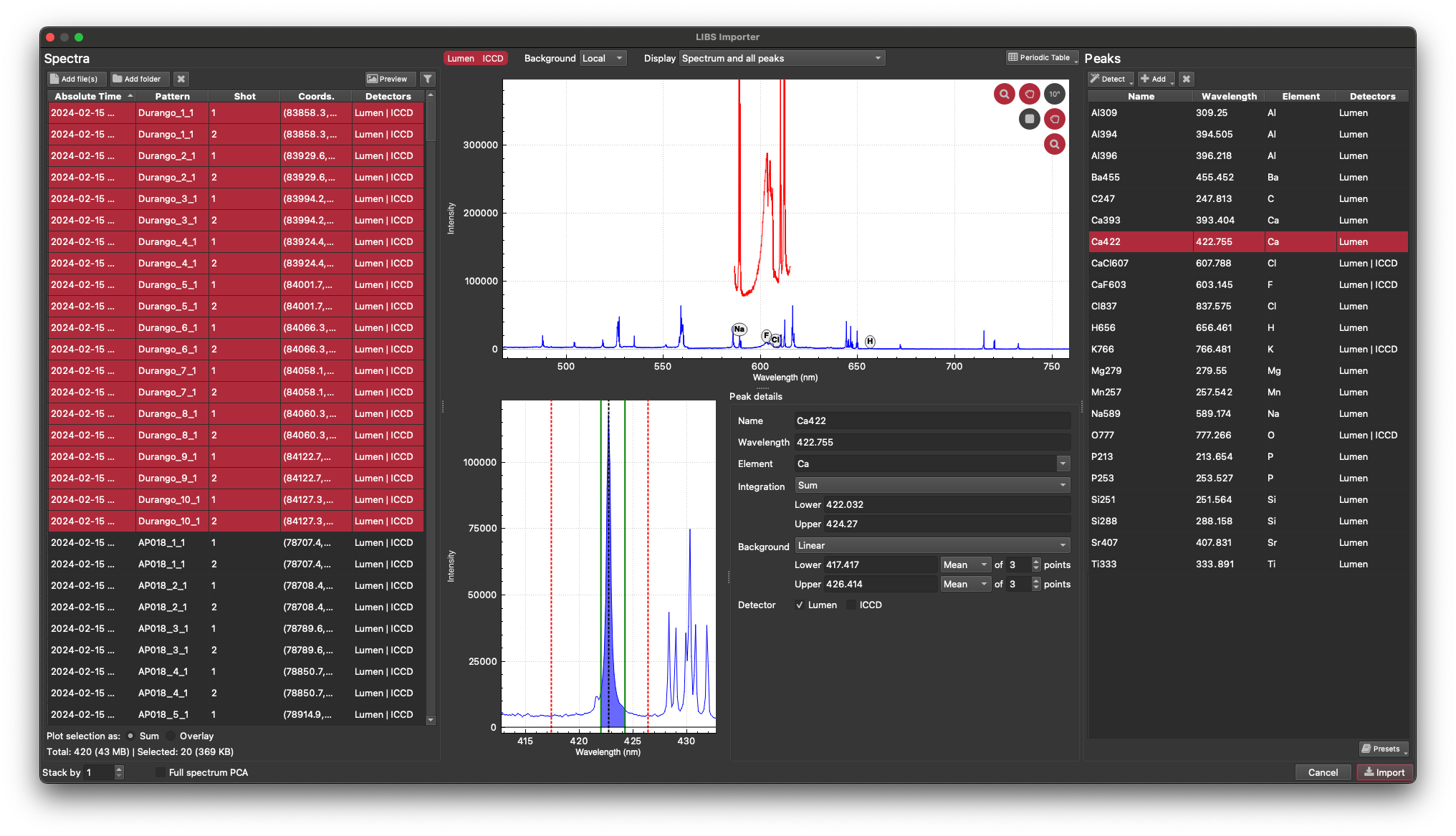
Fig. 26 The LIBS Import Window
The LIBS Import Window
The LIBS Import window has several main parts, shown in Fig. 27. The table of spectra is on the left hand side (empty until a LIBS data file is selected); and central plot showing intensity versus wavelength; a peak detail plot and settings (lower half of central part of window); and a peak list on the left of the window.
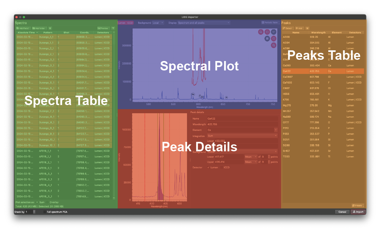
Fig. 27 The four main parts of the LIBS Import Window: The Spectra Table; the Spectral Plot; the Peaks Table; and the Peak Details.
Most parts of the window will be blank/empty until a LIBS data file has been selected, and some peaks have been defined.
Selecting Files and the Spectra Table
A LIBS data file can be opened for inspection, and to start the import process, by clicking the Add file(s) button at the top of the Spectra Table (Fig. 28). This will open a prompt to select an ESLumen .h5 file. You can also open multiple LIBS files by using the Add folder button next to the Add file(s) button. The table of spectra will then be populated with the spectra in the file. You can remove spectra that have been loaded into the table using the button.
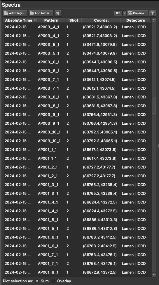
Fig. 28 The Spectra Table
Spectra in the table can be sorted by clicking the column header. The columns shown can be adjusted by right-clicking on a column header and checking which columns you wish to show. You can also filter the list of spectra shown using the button at the top right of the table. This will show a field where you can type in text. Only spectra with Pattern names matching the text will be shown. You can use Regular Expressions in this search field by clicking the .* button to the right of the search field. Clicking the small cross button at the end of the search text field will clear the current search text.
Clicking the Preview button at the top right of the Spectra Table opens the Preview Panel. The Preview Panel is covered in more detail below.
Clicking the 'IFF' button at the top of the Spectra Table performs an Interesting Feature Finding algorithm on spectra in the Spectra Table, as described by Wu et al. (2022). Settings for the IFF algorithm can be set by clicking the down arrow to the right of the IFF button. Options include setting sub-ranges for the IFF algorithm, the number of interesting spectra to highlight, and the number of random features to use in the algorithm (see previous reference for more detail on how the algorithm works). Wavelength ranges can be set in the form 'range-start - range-end', with multiple ranges allowed, separated by commas. For example, to find features in the ranges 200 – 400 nm and 600 – 800 nm, enter '200-400,600-800'.
The result of the IFF is to select the top n most interesting spectra in the dataset. The term 'most interesting' here refers to the number of unique features contained in the spectra. This can make it easier to see which components are present in your dataset and to select peaks.
At the bottom of the Spectra Table are options for plotting (sum of spectra vs overlay; discussed below), information about the total number and file size of spectra loaded, as well as options for stacking spectra and principal component analysis (PCA) options.
If the 'Stack by' field is set to a number greater than one, the integrated data will be downsampled by this factor. For example, setting the 'Stack by' factor to two will halve the number of datapoints in the resulting channels created at import, and each measurement will be the sum of two spectra.
The PCA options are discussed below.
The Spectral Plot
The Spectral Plot is in the upper central part of the window (Fig. 29). Selecting spectra in the Spectra Table will plot their data in the Spectral Plot. You can select individual spectra by clicking on them, or select multiple by clicking on the first you want to select, holding the shift key, and clicking the last you want selected. You can also select all spectra by clicking in the list and pressing Ctrl+A (Cmd+A on Mac), although a maximum of 50 spectra can be selected at any one time (to avoid memory issues).
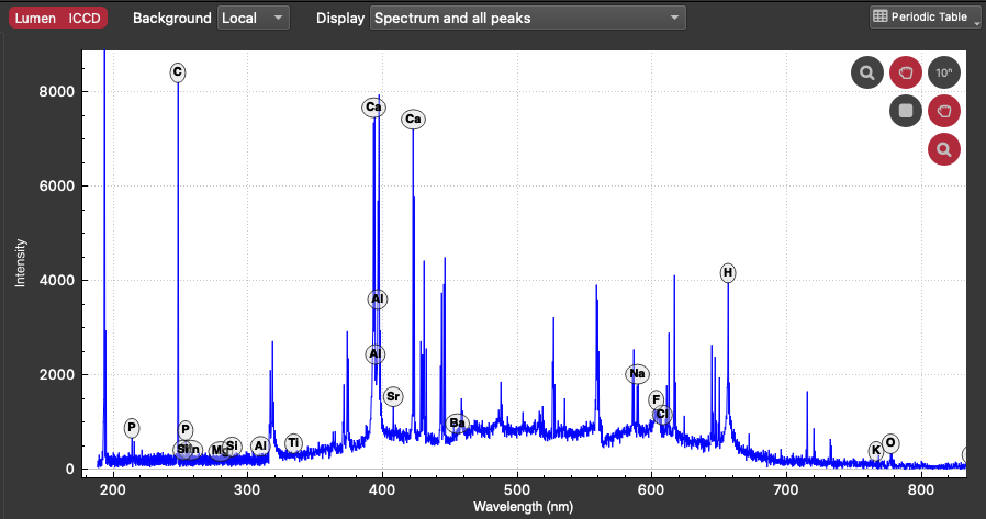
Fig. 29 The Spectral Plot
If multiple spectra have been selected from the Spectra Table, you can choose whether the sum of intensities at each wavelength is plotted (the 'sum') or to overlay each of the spectra in the plot ('overlay') using the Sum and Overlay options at the bottom of the Spectra Table.
The Spectral Plot can be rescaled to show all data by right-clicking on the plot and selecting 'Rescale'. This will rescale both the vertical and horizontal axes to include all available values. You can zoom in on the data using the mouse scroll wheel by toggling the horizontal and/or vertical zoom buttons in the top right of the plot. You can drag the plot data around in the horizontal and vertical axes by toggling the grab buttons in the top right of the plot. Toggling the rectangle zoom button will zoom to a dragged rectangle. Whether the horizontal or vertical axis is zoomed depends on whether the zoom buttons are toggled on or off.
If data for both the Lumen CMOS and iLumen ICCD detectors are available, you can choose whether they are plotted in the Spectral Plot by clicking the 'Lumen' and 'ICCD' button at the top left of the Spectral Plot.
At the bottom of the Spectra Table there are options for plotting the selected spectra as the sum of spectra (the sum of intensities for each wavelength: 'sum') or overlaying each spectrum ('overlay'), showing in Fig. 30. After changing this option, you may need to rescale the Spectral Plot by right-clicking on it and selecting 'Rescale'.
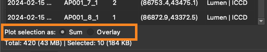
Fig. 30 The Sum and Overlay options at the bottom of the Spectra Table
At the top of the Spectral Plot there are dropdown menus for the Background subtraction and Display options. The Background options are 'None' (no background subtraction), 'Local' and 'Global'. If the 'Local' option is selected, the spectra are background subtracted according to the peak definition (see Peak Details for more information about setting local peak backgrounds). If the 'Global' option is selected, a 'rolling ball' background subtraction approach is taken (e.g. this ref but in one dimension).
The Display options include whether to show just the selected spectra without any peaks identified on the plot (the 'Spectrum' option); the selected spectra and any peaks selected in the Peaks Table (the 'Spectrum and selected peaks' option); the selected spectra and all peaks in the Peaks Table (the 'Spectrum and all peaks' option); and the selected spectra and peaks for elements selected in the Periodic Table panel (see below).
The visible wavelengths can be shown in the background of the Spectral Plot by right-clicking on the plot and selecting the 'Show visible colors' option.
The Periodic Table Panel
Clicking the Periodic Table button at the top right of the Spectral Plot displays the Periodic Table Panel (Fig. 31). This panel shows the elements arranged in the periodic table and elements can be selected by clicking on them. Elements that have been selected have a red border and are a slightly darker color. If the Display option above the Spectral Plot is set to 'Spectrum and peaks for selected elements', the peaks for the selected element will be marked on the Spectral Plot. Each peak for the element is marked with a red line at the peak centre and the height of the line represents the relative intensity of the peak.
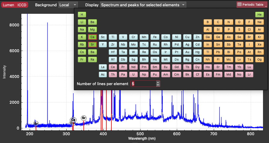
Fig. 31 The Periodic Table Panel, with Ca and Sr selected. Five peaks have been selected for display in the Spectral Plot.
Note
Selecting more than one or two elements in the Periodic Table Panel can make the Spectral Plot quite hard to read. Keeping it to one or two elements at time will make it easier to use.
The number of lines to show per element is set at the bottom of the Periodic Table Panel (default = 10, max of 200) and are ordered by relative intensity.
The Peaks Table and Defining Peaks
The table at the right-hand side of the window is the Peaks Table (Fig. 32). This shows the peaks that have been defined to be integrated when the Import button (bottom right of window) is clicked. There are several ways to add peaks (discussed below). Peaks that appear in the table can be removed by clicking the button at the top.
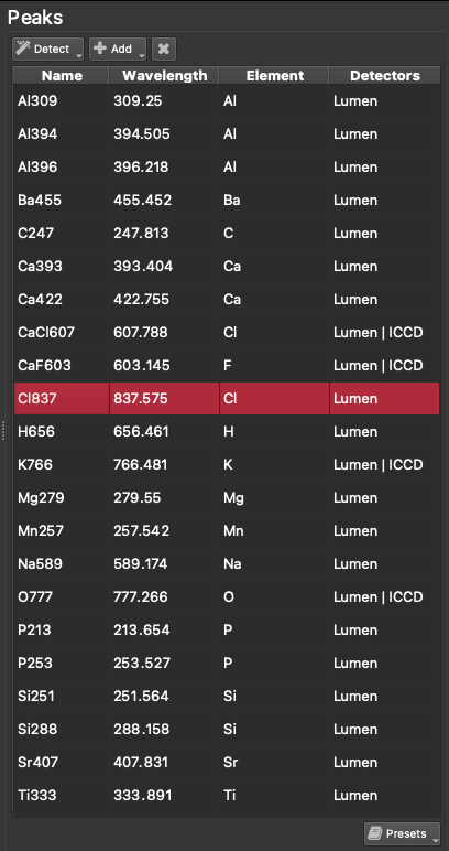
Fig. 32 The Peaks Table, showing a set of defined peaks. The peaks Presets button is at the bottom of the Peak Table
Peaks can be defined in several ways, listed below in order of increasing sophistication. In all cases, peak details can be edited after they have been created using the Peak Details controls. The most basic is zooming into a peak in the Spectral Plot and right clicking on the peak top. The right-click menu includes an 'Add Peak' item that lists the top ten elements (by intensity) with peaks occurring at the wavelength clicked. Selecting an element will add it to the Peaks Table. There is also a 'Custom' option to create a peak at the wavelength clicked, where you will be prompted for the peak name and the element it represents.
Peaks can also be added by clicking the Add button at the top of the Peaks Table. This adds peaks based on wavelength or element. If Wavelength is selected, a wavelength can be entered and the element with the highest intensity at the selected wavelength will be added to the Peaks Table. Selecting the 'By Element' option prompts the user to enter an elements symbol and the number of peaks (n) to add for that element. The highest n peaks for that element will be added to the Peaks Table.
Peaks can be automatically determined by clicking the Detect button at the top of the Peaks Table. The first currently selected spectrum in the Spectra Table is used to determine peaks. If no spectra are selected in the Spectra Table, clicking this button will not define any peaks. The auto-detection algorithm starts by smoothing the intensity of the select spectrum with a five-point box smoothing filter to avoid spikes showing as peaks. A peak is identified if its intensity is above the Intensity Cutoff (default = 2000) and the second derivative of the peak is less than Noise Parameter (default = 100). The Intensity Cutoff and Noise Parameter can be adjusted by clicking and holding down the Detect button until fields showing these values are shown. Intensities are background subtracted using a 'rolling ball' approach before the intensity cutoff is applied. The 'rolling ball' radius is 30 points by default. Click the button at the end of the Noise Parameter field automatically determines the best noise parameter to use, based on the standard deviation of the second deviation of the intensities. This updated value is then displayed in the Noise Parameter field.
Clicking on a Peak in the Peak Table will show it in the Peak Details area in the lower middle part of the window, and in the Spectral Plot if the 'Spectrum and selected peaks' or 'Spectrum and all peaks' Display options have been set for the Spectral Plot.
Peak Presets
A list of defined peaks can be saved for future experiments using the Presets button at the bottom of the Peaks Table. To save the current list of peaks as a new preset, select 'Save current' from the options shown, and provide a name for the preset. To select a previously defined set of peaks, select if from the list.
Selecting the 'Manage' option will show the Presets manager (Fig. 33). Here you can import presets from other users (using the Import button), export presets as .json files to share with others, and rename or delete existing presets.
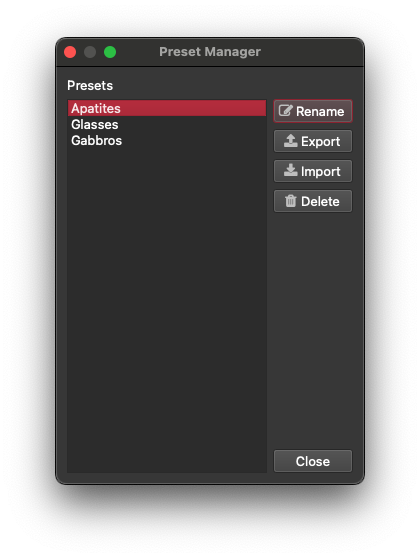
Fig. 33 The Peaks Presets Manager
Peak Details and Peak Plot
The Peak Details displays the name of the selected peak, the wavelength, the element it represents, options for how to integrate the peak, options for background subtracting the peak and the detectors for which the peak is defined (Fig. 34). The Peak Plot (the plot to the left of the Peak Details area) shows a zoomed in region surrounding the plot, and includes lines defining the peak center, integration bounds and background markers (discussed more below).
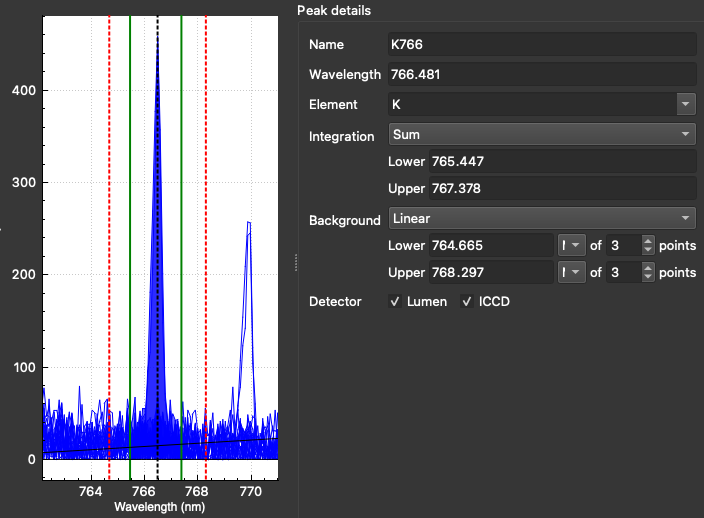
Fig. 34 The Peaks Details area of the LIBS Import Window. The Peak Plot is shown in the left part of the details area. Note that in this screenshot the Background mode was set to 'Local' so the local background controls are visible.
The Name, Wavelength and Element can all be changed by clicking in the respective field and typing (or choosing from the dropdown menu for the Element symbol). The peak wavelength can also be adjusted by clicking and dragging the dashed black line in the Peak Plot.
The interval to be integrated is defined by lower and upper wavelength bounds (in nanometres). These can either be manually typed in using the Lower and Upper fields, or they can be visually adjusted by clicking and dragging the green solid lines in the Peak Plot. Whether the sum or the mean value for the peak is imported can be selected using the Integration dropdown menu.
If the Background Mode (selected using the Background dropdown menu above the Spectral Plot) is set to None or Global, there will be no background settings in the Peak Details. However, if the Background Mode is set to 'Local', the background to be subtracted from the peak is defined by a Lower and Upper point (in nanometres). These can be set using the Background Lower and Upper fields, or visually adjusted by clicking and dragging the dashed red lines in the Peak Plot. The value(s) to be subtracted can either be a linear fit between the upper and lower background values (the default), or a mean or median of values at the upper and lower background values. The value at the upper and lower bounds can be determined from a variable number of points n that can be adjusted using the points fields (default is three points). For a linear fit, the values fit are the mean/median of the upper and lower intervals. Whether it is the mean or median can be changed using the Mean/Median dropdown menu next to the Lower and Upper fields. The black solid line in the Peak Plot shows the background to be subtracted. If the Sum plotting option is selected (at the bottom of the Spectra Table) the solid black line representing the background may not match the plotted data. Changing to the Overlay option will show the background value more clearly.
An integration value can be calculated for one or both Lumen and ICCD detectors using the checkboxes at the bottom the peak information. If both are selected, a channel with the peak label will be created for each detector. For example, if the peak is called 'Ca393', and both detectors are selected, there will be both a 'Ca393_Lumen' and a 'Ca393_ICCD' channel created at import.
Preview Panel
The Preview Panel gives an overview of the integrated values at a selected wavelength. Clicking the Preview Panel button (top right of the Spectra Table) opens the Preview Panel (Fig. 35). By default until a wavelength is selected, the preview panel shows an image created for the midpoint of the spectral range of the selected detector.
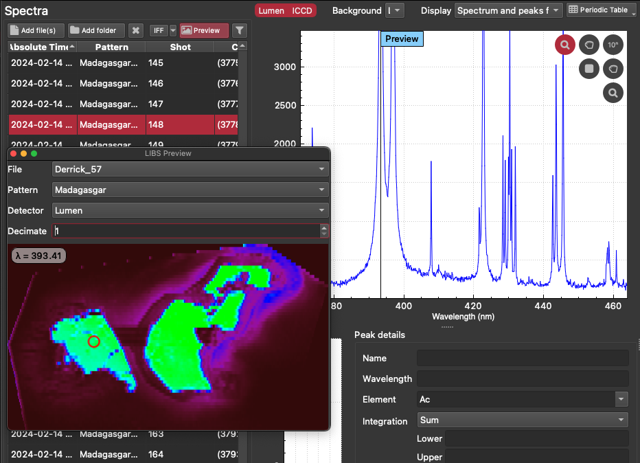
Fig. 35 An example of the Preview Panel, showing the result of integrating the spectra at wavelength 393.41 (selected using the Spectral Plot). In this screenshot, a part of the preview image was clicked (red circle) and the spectrum for this point was automatically selected in the Spectra Table and its data were plotted in the Spectral Plot.
If one or more spectra are selected in the Spectra Table, and the Preview Panel is currently open, a preview line will appear in the Spectral Plot. This line can be clicked and dragged to update the wavelength of Preview Panel's image. Alternatively, to see a preview of an already defined peak, right-click the peak in the Peaks Table and select 'Use for preview'.
The effectiveness of this preview depends on how the patterns in your experiment are set up (patterns with few scanlines/spots will have less information in the preview c.f. those with many scanlines etc.). The pattern to show a preview for can be selected from the Pattern dropdown menu. Similarly, the detector can be selected using the Detector dropdown menu. The 'Decimate' options allows for decimating the spectra used to generate the plot. This can be helpful in experiments with a large number of spectra. By default, only every 5th file is used in the preview.
Clicking on the image in the Preview Panel will select the spectrum corresponding to that part of the image in the Spectra Table, and the data for that spectrum will be plotted in the Spectral Plot. The area clicked is marked by a red circle (e.g. Fig. 35). This can make it easier to find relevant spectra for a particular image/sample.
Principal Component Analysis (PCA)
Principal Component Analysis (PCA) can be used to create channels in iolite from the selected LIBS dataset by clicking the 'Full Spectrum PCA' checkbox at the bottom of the Spectra Table. When this checkbox is checked, controls for the PCA are shown next to the checkbox. These controls allow the analyst to perform the PCA on spectral ranges, whether normalisation of the data is performed before PCA (with options for Z-score and min-max scaling), whether downsampling should be applied to the spectra before the PCA, and how many components to create channels from. The PCA results are only calculated when the Import button is clicked, and the PCA channels created are in addition to the channels created by the defined peaks.
Note
Principal Component Analysis on whole spectra can be very processor intensive and may take quite a while to calculate. Please check your PCA settings before clicking the Import button.
By default the entire wavelength range is used in the PCA, but subranges can be defined. For example, to create channels from PCA of wavelengths 200 to 400 nm, enter '200-400' in Wavelength Ranges field.
To set the amount of smooth downsampling applied before PCA, set the 'S' field. This can decrease the processing time required, but too much downsampling will decrease the sensitivity of the PCA (i.e. features may be missed in overly downsampled datasets).
To set the number of components to create channels for, set the 'N' field. By default, the top five components will be converted to channels.
Importing
Importing the data is performed when the Import button (bottom right of the LIBS Import Window) is clicked. At this time, a new channel is created for each peak in the Peak List (or two channels if more than one detector is selected for the peak e.g. Lumen and ICCD). Each time point in the channel corresponds to a spectrum measurement time, and the data for each measurement is the sum of the peak area after background subtraction (or the mean of the peak area if this has been selected in the Peak Details).
Depending on the size of the .h5 data file and the number of peaks defined, the import process may take a while and no other actions should be taken until the import is complete.
If Principal Component Analysis has been selected, PCA will be performed after the peaks channels have been imported as part of import process. See the PCA section for more details.