Precognition
About
Precognition is an add-on for ActiveView2 (AV2) that can predict measured images given a source image, pattern, acquisition parameters, and single pulse response.
Note
Precognition requires AV2 version 1.5.0.25 or later.
How it works
Precognition uses the laser pattern information, along with the modeled cell response and a base sample image, to generate time series data. These time series data are sampled according to the mass spectrometer's acquisition parameters, and the result is input into iolite's image generation algorithms to create a predicted image. The base image can be any image of the sample such as a photomicrograph or SEM image etc, but should be at sufficient resolution to see the features of interest in your sample (without being excessively detailed or an excessively large image file). It is important to note that the prediction is not trying to model what the trace element distributions will be exactly, but to give the operator a sense of what level of detail would be available if the current analytical settings were used.
Precognition will also provide warnings if it identifies potential issues with the analytical parameters. These include image aliasing (frequency effects between the mass spec sampling frequency and the laser ablation rate); issues with the laser or mass spec settings (e.g. scanning the laser too quickly, or insufficient dwell time for low signal to noise elements); as well as providing overall information about the experiment such as spot overlap, pulse dosage and total analysis time.
Installation
Obtain the installer from the iolite store
Run the installer on your AV2 computer
Activate the Addin using ActiveView2's Settings (the cog button, bottom left) -> Manage Addin
Install and register iolite 4 on the ActiveView2 computer (see the iolite installation guide for installation details)
General workflow
The general workflow begins by importing your base image and aligning it with the main video image in AV2. Then a pattern is created over the image, using a first guess at the ideal ablation parameters (spot size, scan speed, line spacing etc). Once an image and pattern have been added, you can then open the Precognition panel by clicking the + symbol on the left. The user interface is described below. A pattern and image is selected, and the mass spectrometer settings are entered. A model cell response is chosen, and a prediction can then be made. After the prediction is completed Precognition will show some suggestions and warnings. Depending on the outcome of the prediction and the suggestions, you may want to go back and change your ablation pattern parameters or mass spec settings. You can also use one of Precognition's optimisation routines to automatically adjust the mass spec settings, and then predict a new outcome with the new settings.
If you've changed the mass spec settings, after you're happy with the prediction, you can then update your mass spec method if you've made any changes to your acquisition paramters.
Usage
The user interface for Precognition is shown below where the workflow generally moves from the top to the bottom.
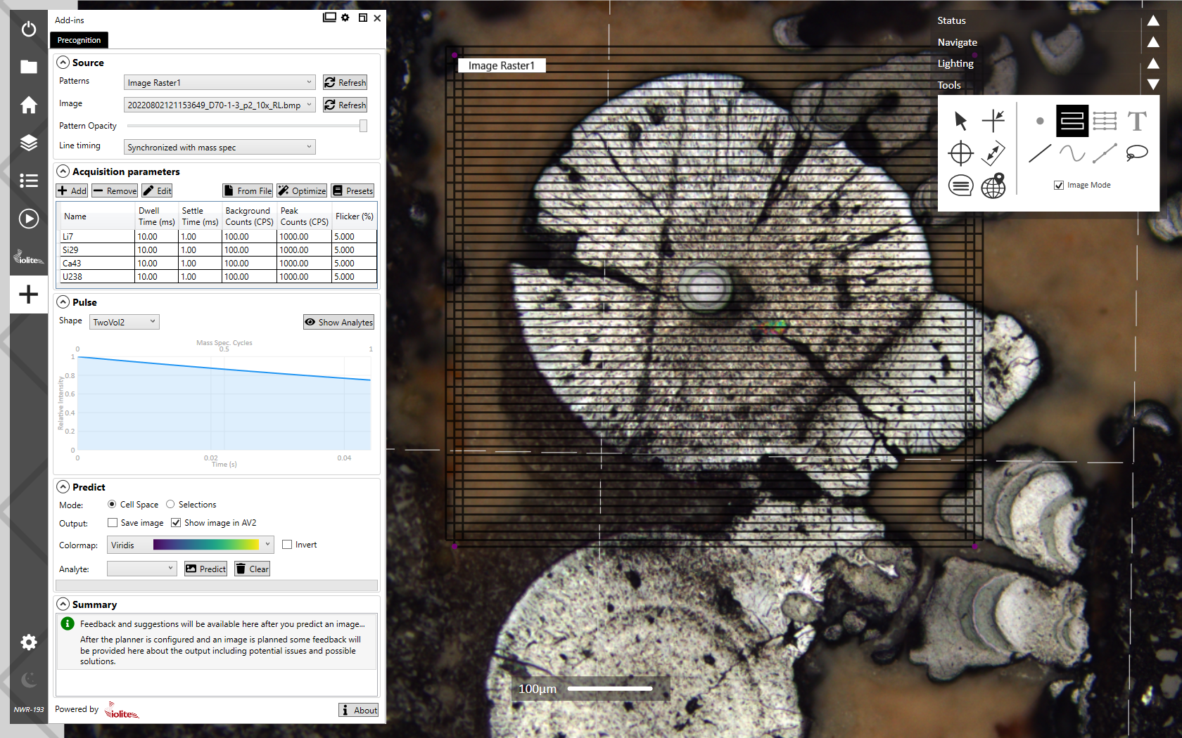
There are five main panels for setting up the prediction, discussed below. Each panel is expandable/collapsible using the arrow button next to the panel's title. The output predicted image will be shown in the main image area of AV2 and/or saved to file, based on your settings.
Source
The Source panel allows you to choose which pattern you have defined in AV2 to predict an image for. You can also select your base image here.
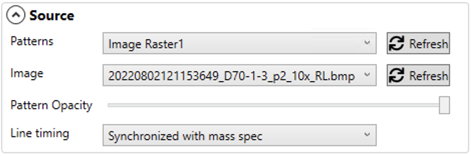
After a pattern is added, using AV2's normal pattern creation tools, click the Refresh button so that the pattern appears in the dropdown list in Precognition.
The source image is used to adjust the count rates in the prediction: areas that are light in the source image will have corresponding high count rates in the predicted image and vice versa for dark areas in the source image. This is necessary as otherwise the output image would all be one countrate and it would be impossible to tell what level of detail is observable.
The Pattern Opacity slider adjusts the ablation pattern's opacity over the predicted image, and is mostly used after a prediction has been completed.
The Line timing options are provided to adjust how the mass spec sampling will proceed at the start of each line. The 'Synchronized with mass spec' option is used where the mass spec will start at the same point in its collection cycle for each line scan. The 'Fixed delay' option allows for a specified amount of time between the end of the previous line and the start of the next, during which the mass spectrometer is still cycling. The 'Random delay' option is for a random amount of time elapsed between the end of one line and the start of the next. The latter option is best when there are various distances between the scanline lengths, whereas if the scanline lengths are all the same and the mass spec data is collected in a single file, the 'Fixed delay' option may be more appropriate. If a new mass spec sample is started with each new scanline, the 'Synchronized with mass spec' option may be best. If unsure, use the 'Synchronized with mass spec' option.
Note
It is important to note that all predictions will be offset from the observed/measured data: the question is by how much. Using an approximation here may still provide you with some indication of the success of your experiment, even if it is an approximation.
Acquisition Parameters
The Acquisition Parameters panel is where the mass spectrometer sampling paramters are set up. The table of channels measured displays the name of the channel, the dwell and settling time, the background and peak (on sample) count rates, and the flicker (noise) for each channel (see figure below).
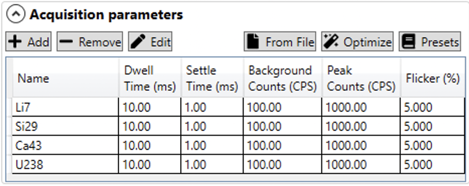
You can manually add analytes using the Add button. By default the new analyte will be labelled "Si29" and have a dwell time and settling time of 10 and 1 ms, respectively. The default background counts is 100 CPS, and the default on peak counts is 1000 CPS. The default flicker is 5%.
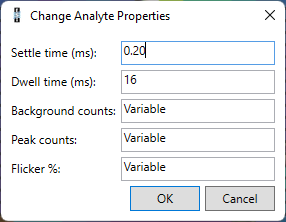
You can remove any analyte by clicking it in the table and clicking the Remove button. You can edit any of the values for an analyte by clicking on it in the table. If you would like to change the value for multiple analytes at once, you can select the analytes and click the Edit button. In the dialog that appears, you can set the value for all the selected analytes.
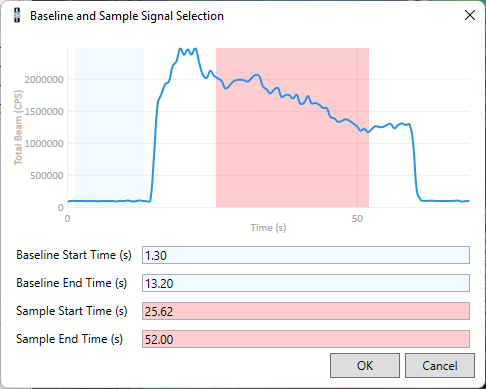
The prediction will be more accurate if you measure a test scanline and import the results into Precognition. The test scanline could be across a part of the sample not included in the main area to be imaged, or across a sample with similar composition to your actual sample. You can then load this test data using the From File button. Currently you can load data from Thermo iCap, Perkin Elmer Nexion, and Agilent quadrupole instruments. A window will appear where you can select representative background (blue) and peak (pink) regions (shown below). You can adjust the default periods by clicking the left or right edges of the blue or pink rectangles, or by changing the values displayed below the graph. You can zoom the displayed data in or out using the mouse scroll wheel. You can move the data left or right by clicking it and dragging it left or right. Once you have selected the representative background and sample regions, click the OK button, and the analytes will be added to the analytes table.
When using an iCap .csv or Nexion .nc file, the dwell times will be imported automatically. If you import a .csv file from within an Agilent batch folder, Precognition will read the dwell times from the .xml files in the same folder. Settle times are automatically calculated as the difference between the sum of the dwell times and the total cycle time, divided by the number of analytes.
Precognition will calculate the mean and uncertainty for the selected background and sample regions and add these to the analytes table.
Once you have set up your analytes, you can save the set as a preset for future experiments by clicking the Presets button. You can also load preset analyte sets using this button.
Analysis Optimization
Precognition offers three optimisation strategies for optimising the dwell times for each analyte. These are 'Hutchinson', 'van Malderen' and 'Even'.
Hutchinson method
The Hutchinson method attempts to reduce the dwell times while maintaining the statistical difference between the background and peak signal, given the current analyte background and peak counts and dwell times. For example, if you have an analyte with significant difference between the peak and background, you may be able to decrease the dwell time to reduce your overall cycle time. You can set the number of standard deviations between the peak and background using the Sigma parameter. You can also add additional 'breathing space' between the two populations (peak and background) using the 'Breathing space' parameter. As this method aims to reduce the dwell time based on the observed counts, it may reduce the dwell times to values that result in very low duty cycle (the amount of time spent collecting data relative to the total cycle time). You can avoid this by setting a minimum dwell time. For more than one or two analytes, we would recommend dwell times of no less than 10 ms. If your mass spec allows setting fractional dwell times, you can check the fractional dwell times checkbox to avoid having to use whole millisecond dwell time values. However, this may result in dwell times just slightly lower than the specified minimum dwell time.
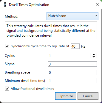
To avoid frequency effects between your laser firing rate and your mass spec cycling time, you can choose to synchronize your total cycle time with some multiple of the laser repetition rate using the 'Synchronize cycle time to rep. rate' checkbox. If this value is set to one, the optimisation will attempt to fit all masses between one pulse of the laser and the next. If this results in very short dwell times where the mass spec duty cycle is too low, you can expand the number of cycles using the Cycles parameter. For example, by default this parameter is 1 and all masses will be fit into one laser pulse. Increasing this to 3 will fit the total cycle time into three pulses of the laser, allowing for longer dwell times and more reasonable duty cycles.
van Malderen method
The van Malderen method distributes the dwell times within the total cycle time according to the inverse of the signal to noise ratio (SNR) of each analyte. You can set how many pulses of the laser the total cycle time should be synchronized with using the 'Synchronize cycle time to rep rate ' checkbox, and you can set the minimum dwell time using the 'Minimum dwell time' parameter.
Even method
This method simply distributes the dwell times for all analytes evenly within the total cycle time, while synchronizing with the laser repetition rate. You can set the number of cycles to synchronize with the laser pulses, as well as the minimum dwell time.
Note
After you have run an optimisation, the background and peak count rates and flicker values displayed in the analytes table will no longer reflect what would be expected from a measurement with the displayed dwell times. That is, if you have decreased your dwell times you may have also increased your uncertainty for both background and peak count rates. You should not run another optimisation until you have measured another test scanline using the suggested dwell times to update the background and peak values.
Pulse
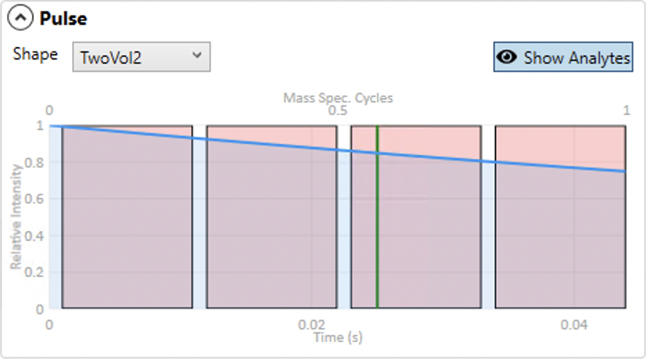
The Pulse panel allows the analyst to specify the model cell response from a single laser pulse. There are several presets for ESL cell types, as well as four numeric models that can be adjusted by changing the 'A' parameter (except the 'Ones' model that results in a steady state signal regardless of the A parameter). It should be noted that all of these are approximations of the actual cell response. Future versions of Precognition may include the ability to measure the cell response of your system and load it into Precognition to use in the prediction process.
Clicking the Show Analytes button will overlay the position of the analytes over the cell response graph, assuming the mass spec cycle starts exactly at the start of the pulse. This allows you to see how the dwell times are distributed. If, for example, one analyte has a longer dwell time due to lower SNR, it will show as a wider measurement time in this graph. Vertical green lines in this graph show the position of subsequent laser pulses so that you can see where each analyte will be in the washout cycle. These will only show if your total cycle time is longer than the period between two laser pulses. Not shown is the signal increase and then washout after each subsequent laser pulse.
Predict
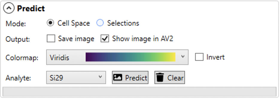
The Predict panel is where the prediction options are set. You can choose between assembling the image data as a CellSpace image or an Image by Selections. The latter is constructed where each mass spec measurement is a pixel in the resulting image, whereas a CellSpace image arranges mass spec measurements according to the laser's x, y position and spot size when the measurement was made. CellSpace images may have overlapping spots which can increase the apparent resolution of the image. See the link above for a full description of the CellSpace method of image creation.
Typically the predicted image will be shown in the main display of AV2, although this can be toggled on or off using the 'Show image in AV2' checkbox. A copy of the predicted image can be saved to disk by checking the 'Save image' checkbox. The color map of the predicted image can be set here, along with which analyte is predicted (only one analyte at a time is predicted).
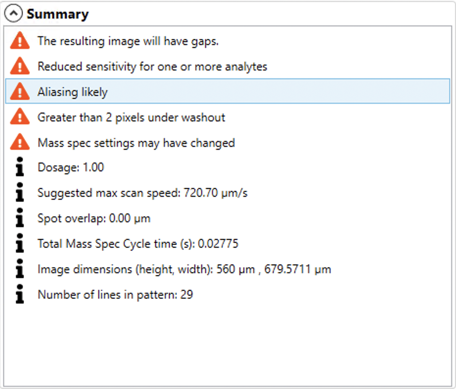
Summary
The Summary panel shows any suggestions and warnings based on your combination of cell response, laser pattern and acquisition settings.
Clicking on any warning (shown with an orange icon) will show some more detail about that warning. Information related to the experiment, such as dosage, spot overlap and final image dimensions are also shown for reference and consideration in planning your experiment.
If you do change any of the mass spec or laser settings, you can re-run the prediction to see the effect. For example, if Precognition recommends that you could increase your laser scan speed, you can go to the pattern in AV2's normal pattern editing interface (e.g. by right-clicking on the pattern and selecting Properties) and update the overlap to increase the scan speed. You can then go back to Precognition, click the Refresh button to update the pattern parameters and repeat the prediction. The updated prediction will show the effect of increasing the scan speed.
Note
The suggestions shown by Precognition only take into account the information provided and use the estimates described above. Hence they are just suggestions and the analyst may subsequently make informed decisions about which suggestions they use in their experiment setup.
Support
If you have any problems, suggestions or questions, please do not hesitate to contact us at support@iolite-software.com.