Notes
This content is auto-generated from the notes site. There may be formatting issues as it is transcribed.
Python integration
If you are using iolite 4, you've probably noticed references to something called 'python' in the user interface. Python is a general purpose interpreted programming language widely for many things, but has become particularly popular among scientists for data processing and analysis. iolite 4 has a built-in python interpreter that you can use for a variety of tasks and one of the main goals of iolite notes is to educate our users on the various ways we can harness its power to do something interesting.
More about python
Like all programming languages, python has a specific syntax. To acquaint yourself with python syntax you can refer to any number of external resources, such as:
And for the more data/math/science oriented stuff: SciPy Lecture Notes.
Libraries, packages and friends
iolite 4 is built with Qt, and a great deal of that functionality is available to you through iolite's use of PythonQt. More information about the Qt and PythonQt application programming interface (API) and functionality is readily available online.
Python is known for its many packages. iolite is distributed with many useful data science packages such as:
And more!
It is also possible to add your own packages to be used with iolite's python interpreter. More on that later!
The python "API"
The API is described in the online iolite documentation. A few basics are outlined below to give you an idea how it works.
Getting a selection from a selection group:
sg = data.selectionGroup('G_NIST610')
s = sg.selection(0)
Doing something to each selection:
sg = data.selectionGroup('G_NIST610')
for s in sg.selections():
    doSomethingWithSelection(s) # Where the function doSomethingWithSelection has been defined elsewhere
Getting the data and time arrays from a channel:
c = data.timeSeries('U238')
d = c.data()
t = c.time()
Note: if you try to get a selection group or channel that does not exist, python will raise an exception, e.g.
- Traceback (most recent call last):
File "
", line 1, in RuntimeError: std::runtime_error: [DataManager::timeSeries] no matches for ...
Integration in iolite
We have integrated python in several places, not all of which are obvious, so let's review the various ways python can be used now.
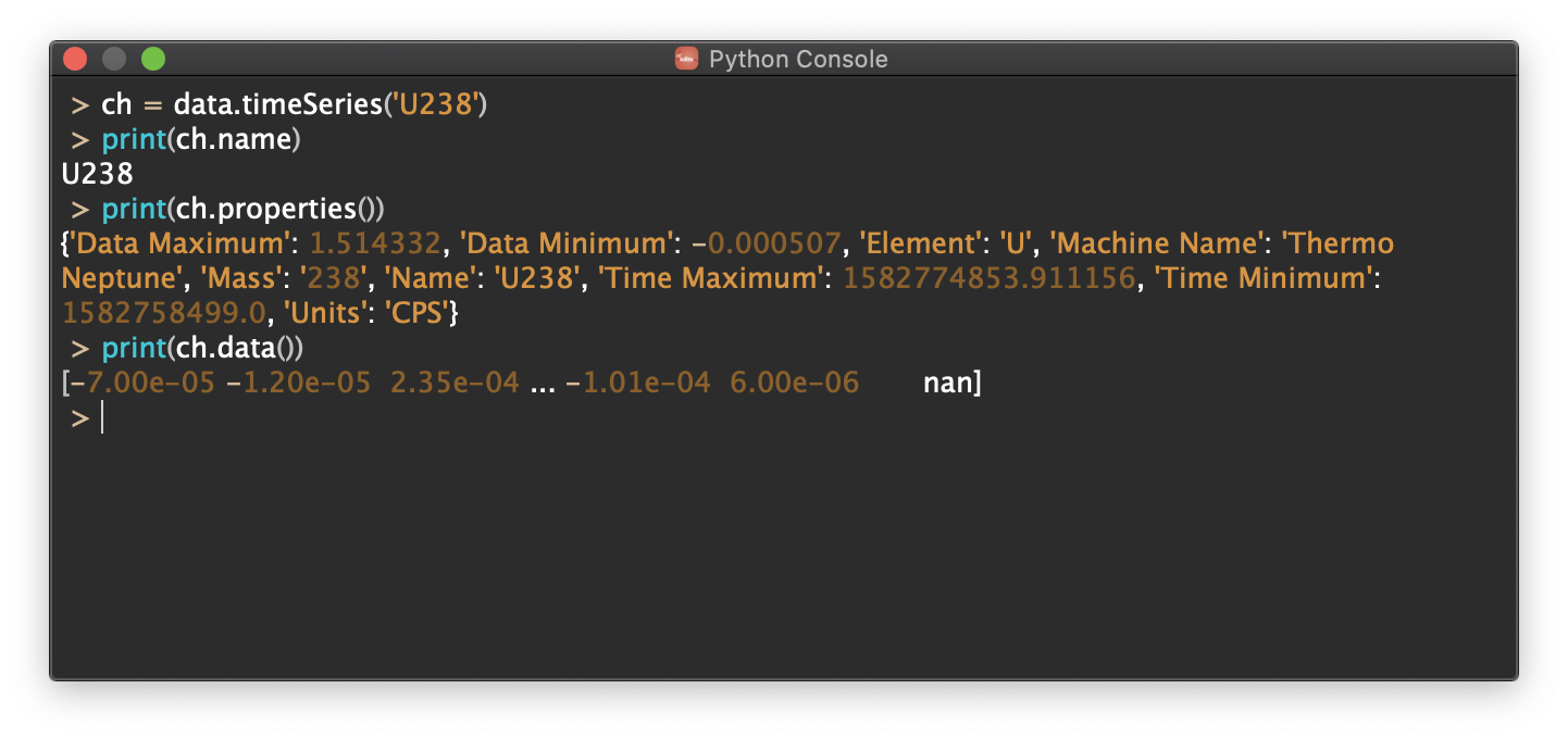
Console
This is a place to type in a quick command or short series of commands that you are not likely to do often. It can be accessed from the Tools menu as Python Console or from the keyboard short cut CTRL+SHIFT+P (PC) or CMD+SHIFT+P (Mac).
Workspace
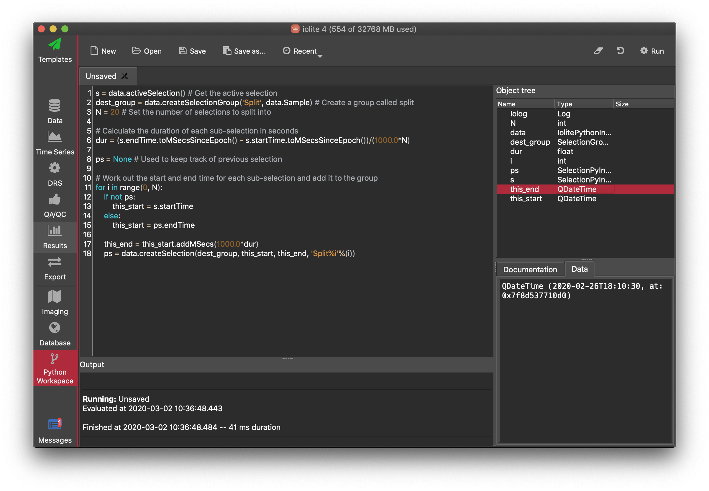
This is a place to write small (or large!) reusable scripts that are not suitable to be written as a plugin (see below). It can be accessed from iolite's toolbar on the left side of the main window.
Plugins
We have also included the ability to write plugins or add ons for iolite by including specific metadata in your python file and putting the file in the location configured in iolite's preferences.
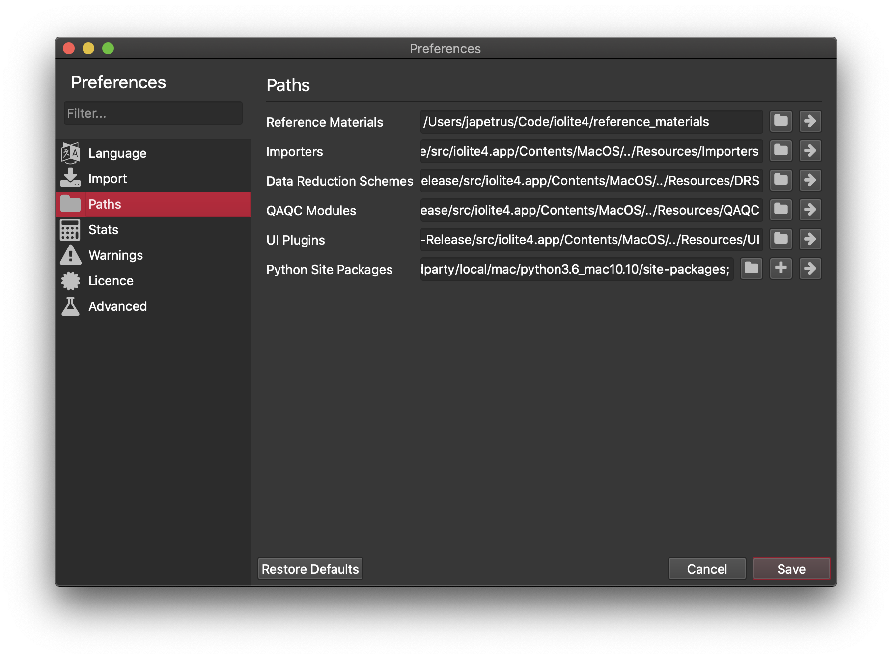
Note that by default these paths are within the main program folder (i.e. in Program Files for Windows and /Applications/iolite4.app for Mac). This is convenient, but problematic (see below). If you want to keep iolite up to date (recommended) and have your own add ons and/or reference material files, you should change these paths to a separate folder (e.g. in your Documents).
Python plugin types that required extra metadata include importers, data reduction schemes, QA/QC and user interface (UI). The meta data generally looks something like this:
#/ Type: DRS
#/ Name: U-Pb Python Example
#/ Authors: Joe Petrus and Bence Paul
#/ Description: Simple U-Pb with downhole fractionation corrections
#/ References: Paton et al., 2010 G3
#/ Version: 1.0
#/ Contact: support@iolite-software.com
In addition to the metadata, certain functions are also required and vary depending on the plugin type. This metadata and the required functions allow iolite to parse these files and insert them into the user interface as appropriate. For example, a DRS needs to have functions runDRS and settingsWidget. To learn more about plugins and their format you can visit our examples repository on github.
Other places
There are a few more places that python can be used in iolite, including to write custom export scripts (e.g. if you wanted to output certain columns in a certain format and did not want to fuss with it after exporting), within processing templates (e.g. if you wanted to check for outliers within selection groups and move them to a different group, or to perform some custom QA/QC). The calculator tool also uses python to evaluate each expression and therefore python syntax and benefits apply.
Potential problems
Since some parts of iolite depend on python, if the path to python packages is not configured properly in iolite's preferences, iolite may not be able to start. If that happens, you can hold down shift while starting iolite to reset some of the preferences to their default value.
Since the paths for python-based add ons are within the program folder by default, you may encounter problems when trying to create a new add on from the iolite interface because the operating system may prevent you from creating new files in those locations.
Additionally, if you have modified files in the default paths be warned that these files will be lost when updating!
Click here to discuss.
Manipulating selections from python
A reminder about selections
A selection in iolite is simply a named (and grouped) period of time. Data processing in iolite revolves around groups of these selections and groups of different types. A selection's period of time is defined by a start time and an end time. Of course things can be more complicated when you throw in linked selections and other properties, but for now let's consider a few ways we can manipulate selections with python.
A reminder about python
Python is a programming language that you can write add ons and other scripts in for iolite 4. To read more about python and the various ways you can use it in iolite, see here.
Examples
Adjusting all the selections in a group
# first we get the desired selection group by name and assign it to a variable called 'sg':
sg = data.selectionGroup('GroupName')

# then we use a for loop to iterate over all the selections in the group:
for s in sg.selections():
    s.startTime = s.startTime.addSecs(2)
Creating selections based on some arithmetic
from iolite.QtCore import QDateTime

# Establish a start time using a specific format
start = QDateTime.fromString('2020-02-06 12:00:00.000', 'yyyy-MM-dd hh:mm:ss.zzz')
# Create a group named "TestGroup" of type "Sample"
group = data.createSelectionGroup('TestGroup', data.Sample)
duration = 20 # Selection duration in seconds
gap = 2 # Gap between selections in seconds
N = 30 # Number of selections to create

# Create the selections according to the parameters above:
for i in range(0, N):
    this_start = start.addSecs(i*(duration + gap))
    this_end = this_start.addSecs(duration)
    data.createSelection(group, this_start, this_end, 'Sel%i'%(i))
Split selection into several sub selections
s = data.activeSelection() # Get the active selection
dest_group = data.createSelectionGroup('Split', data.Sample) # Create a group called split
N = 20 # Set the number of selections to split into

# Calculate the duration of each sub-selection
dur = (s.endTime.toMSecsSinceEpoch() - s.startTime.toMSecsSinceEpoch())/(1000.0*N)

ps = None # Used to keep track of previous selection

# Work out the start and end time for each sub-selection and add it to the group
for i in range(0, N):
    if not ps:
        this_start = s.startTime
    else:
        this_start = ps.endTime

    this_end = this_start.addMSecs(1000.0*dur)
    ps = data.createSelection(dest_group, this_start, this_end, 'Split%i'%(i))
Click here to discuss.
Downsampling and exporting time series data
We recently had an email asking about exporting time series data that had been smoothed by averaging. It turns out this is something very easy to do with iolite 4's built in python interpreter. Before continuing, if you are not familiar with iolite's python functionality you may want to check out this post first.
Step by step
Getting access to a channel's data and time in iolite via python is as easy as:
d = data.timeSeries('U238').data()
t = data.timeSeries('U238').time()
This gets us the data/time as NumPy arrays. Now downsampling this data by averaging can be done as follows:
import numpy as np
ds = np.mean(d.reshape(-1, 4), 1)
where the 4 means we will average 4 points together. However, this assumes that the length of your data array is divisible by 4. To make things a bit more generic, we could write it as follows:
def downsample_for_export(data_array, n):
    end = n * int(len(data_array)/n)
    return np.mean(data_array[:end].reshape(-1, n), 1)

ds = downsample_for_export(d, 4)
To demonstrate that this works, we can plot the before and after for a specific selection:
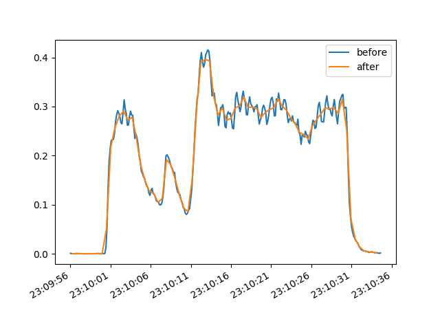
Saving the data is also easy using NumPy (delimited, e.g. csv) or pandas (many formats, including Excel):
np.savetxt("/Users/name/Desktop/file.csv", ds, delimiter=",")

import pandas as pd
pd.DataFrame(data=ds).to_excel("/Users/name/Desktop/file.xlsx", index=False)
Now suppose we want to be able to specify the amount of time for each data point rather than the number of data points. We could do that by inspecting the time array:
tdelta = np.diff(t).mean()
n = int(time_per_point/tdelta)
If we wanted to do it for every channel without needing to specify their names, we could use a for loop as follows:
for channel in data.timeSeriesList():
    ds = downsample_for_export(channel.data(), time_per_point)

    ...
Lastly, we can also bring in some Qt dependencies to make things a bit more user friendly:
from iolite.QtGui import QFileDialog, QInputDialog
time_per_point = QInputDialog.getDouble(None, "Time per point", "Time per point", 1)
filename = QFileDialog.getSaveFileName()
Putting it all together
Combining everything above into one neat little script that will ask us what we want for the time per point and where to save the data looks like this:
import numpy as np
import pandas as pd
from iolite.QtGui import QFileDialog, QInputDialog

def downsample_for_export(channel, time_per_point):
    d = channel.data()
    t = channel.time()

    tdelta = np.diff(t).mean()
    n = int(time_per_point/tdelta)
    end = n * int(len(d)/n)

    return (np.mean(t[:end].reshape(-1, n), 1), np.mean(d[:end].reshape(-1, n), 1))

tpoint = QInputDialog.getDouble(None, "Time per point", "Time per point", 1)

columns = ["Time"]
data_ds = []

for channel in data.timeSeriesList():
    t_ds, d_ds = downsample_for_export(channel, tpoint)
    if not data_ds:
        data_ds.append(t_ds)

    columns.append(channel.name)
    data_ds.append(d_ds)

filename = QFileDialog.getSaveFileName()

df = pd.DataFrame.from_items(zip(columns, data_ds))
df.to_excel(filename, index=False, sheet_name="Downsampled data")
Note that now my downsample_for_export function returns a tuple of time and data so that the downsampled time can be used for plotting purposes. Also note that time in iolite is stored as "time since epoch" in seconds. See here for more info, but it is essentially the number of seconds since 1970-01-01 00:00:00.000 UTC.
How I made the plot
import matplotlib.pyplot as plt
import numpy as np
import matplotlib.dates as mdate

s = data.selectionGroup('Demo').selection(0)
U = data.timeSeries('U238').dataForSelection(s)
t = data.timeSeries('U238').timeForSelection(s)
t = mdate.epoch2num(t)

def downsample_for_export(data_array, n):
    end = n * int(len(data_array)/n)
    return np.mean(data_array[:end].reshape(-1, n), 1)

plt.clf()
fig, ax = plt.subplots()
plt.plot_date(t, U, "-", label='before')
plt.plot_date(downsample_for_export(t, 4), downsample_for_export(U, 4),"-", label='after')
date_formatter = mdate.DateFormatter("%H:%M:%S")
ax.xaxis.set_major_formatter(date_formatter)
fig.autofmt_xdate()
plt.legend()
plt.savefig('/Users/japetrus/Desktop/demo.png')
Click here to discuss.
Accessing session data from 3rd party software
In iolite 3, sessions were saved as Igor Pro "packed experiment" pxp files. This was convenient because iolite 3 was built on top of Igor Pro. The main downside to this was that Igor Pro pxp files cannot be easily read by most 3rd party software. In iolite 4, sessions are saved as files with an "io4" extension. However, this extension is just for show as the data format of the file is actually HDF5. This is super convenient because many scientific data analysis and plotting packages support the HDF5 format.
As an example, let's go through how you can load data from an iolite 4 session file into Igor Pro to be plotted.
Making Igor Pro aware of HDF
Igor Pro comes with all the tools to enable HDF interaction but it does not enable them by default. To enable Igor's HDF functionality (for Igor Pro 8 64bit, others may differ):
Go to the Help -> Show Igor Pro Folder menu item.
Go to the Help -> Show Igor Pro User Files menu item.
Navigate to "More Extensions (64-bit)/File Loaders" in the Igor Pro folder, find "HDF5-64.xop" and copy it (or make a shortcut to it).
Paste "HDF5-64.xop" in the "Igor Extensions (64-bit)" folder in the User Files folder.
Navigate to "Wavemetrics Procedures/File Input Output" in the Igor Pro folder, find "HDF5 Browser.ipf" and copy it (or make a shortcut to it).
Paste "HDF5 Browser.ipf" in the "Igor Procedures" folder in the User Files folder.
Restart Igor Pro.
That's it. You should now be able to access the HDF data browser by going to the Data -> Load Waves -> New HDF5 Browser menu item in Igor Pro.
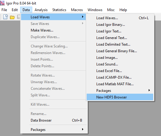
Importing some data
When you activate the "New HDF5 Browser" menu item, you will be greeted by a dialog that looks as follows:
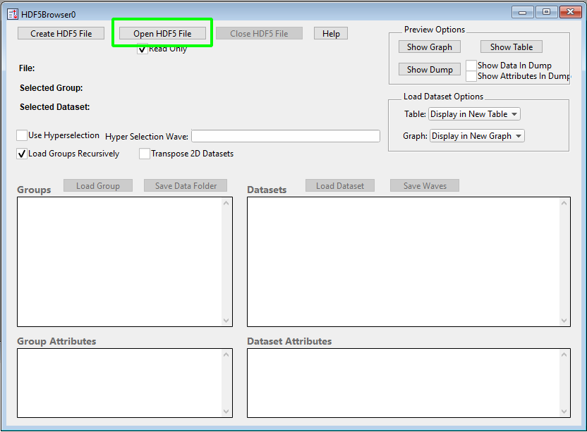
To start, we click the highlighted "Open HDF5 File" button and select the iolite 4 session file we want to get some data from. Once the file is loaded, you can navigate the various groups on the left and datasets on the right. Once you have found a channel you want to plot, you can select it and lick the "Load Dataset" button highlighted below.
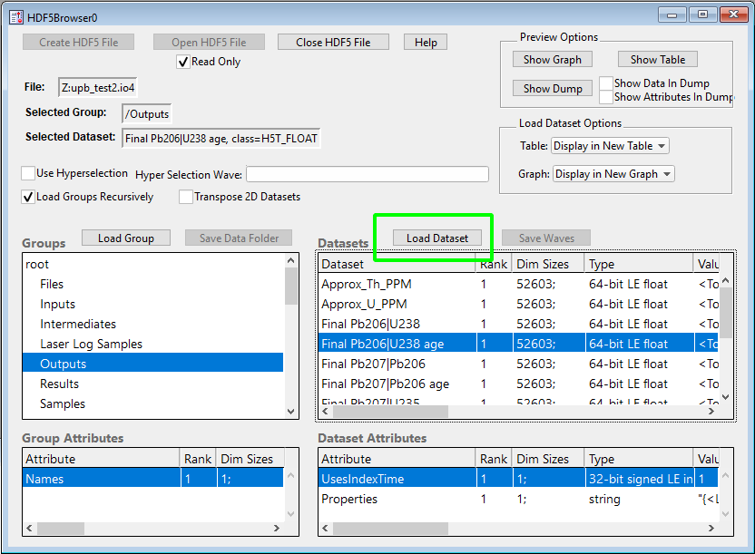
You may need to repeat this process a few times to get all the channels you want loaded into Igor Pro. Also note that some channels use "IndexTime", which you can find in the "Special" group.
Adjusting the time
Igor and iolite handle time a bit differently. If it matters to you that the time axis is the true value, you'll want to adjust it as follows (e.g. in the Command Window - Ctrl+J or Cmd+J):
IndexTime += Date2Sec(1970, 1, 1)
Making a plot
Now that you have the channel and time data loaded, you can make a plot in the usual Igor Pro way. You can start by going to the Windows -> New Graph menu item and selecting the time as X and the channel as Y. I chose one of the final age outputs to plot and made some adjustments to the style:
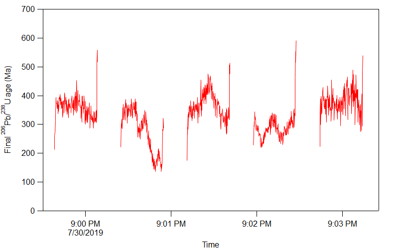
Click here to discuss.
Installing additional python packages
iolite comes with many useful python packages, but we cannot anticipate everything our users might want to use python for in iolite. If your great idea depends on additional python packages that we do not include, here is a quick overview of one way you can install those packages.
Typically the Python Package Index is the best place to start if you know which package you're looking for. You would start by searching for the package, clicking the Download files link on the left side under Navigation and downloading the appropriate file for your operating system and python version.
This is where we encounter the first possible complication. Python packages that are pure python (no machine/operating system specific code) are easy and will normally be provided as a single .whl or zip file. Python packages that are not pure python are a bit tricker and require you to know which version of python you are using (version 3.6 is embedded in iolite at the time of writing but may change in the future) and which operating system / architecture you are using. As an example for the latter scenario, let's look at the files available for SciPy. The format generally looks like:
scipy-VERSION-cpPYTHONVERSION-cpPYTHONVERSIONm-OSINFO.whl
Where VERSION is the package version (1.4.1 as I write this), PYTHONVERSION is 36 and the OSINFO might be something like win_amd64 or macosx_10_6_intel. So, for this particular example, the files we would want to download would be scipy-1.4.1-cp36-cp36m-win_amd64.whl for PC and scipy-1.4.1-cp36-cp36m-macosx_10_6_intel.whl for Mac.
Note that this technique does not do any dependency resolution. For example, if package A depends on package B and you've installed A as above, you will also need to install package B.
An example
As an example, let's install SymPy, a symbolic mathematics package. When we search the Python Package Index and go to the SymPy download files there are two versions: a .whl file and a .tar.gz. A .whl file is a python package format that is essentially a zip file and the .tar.gz is a also a compressed archive, but one not commonly used on Macs and PCs. If we download the .whl version, we could simply rename it to .zip, extract it and copy it to our python site-packages. The location of your site-packages can be found in iolite's preferences. However, do note that you can also add a location outside of the application installation directory if you do not want these packages replaced every time you update iolite.
Alternatively, a simple python script runnable from the python workspace can be used to install .whl files:
from iolite.QtGui import QFileDialog, QMessageBox
import zipfile
import sys

whl_file = QFileDialog.getOpenFileName()
site_path = [p for p in sys.path if 'site-packages' in p][0]

button = QMessageBox.question(None, 'Install Wheel', 'Are you sure you want to install:\n%s\nto\n%s?'%(whl_file, site_path))

if button == QMessageBox.Yes:
    with zipfile.ZipFile(whl_file, 'r') as zip_ref:
        zip_ref.extractall(site_path)

    QMessageBox.information(None, 'Install Wheel', 'You will need to restart iolite before you can use the new package')
Now if you try to import the sympy package in iolite, for example:
from sympy import *
# or
from sympy import expr
you will likely see an error as follows:
ModuleNotFoundError: No module named 'mpmath'
During handling of the above exception, another exception occurred:
- Traceback (most recent call last):
File "
", line 1, in File "/Applications/iolite4.app/Contents/Frameworks/python3.6/site-packages/sympy/init.py", line 21, in raise ImportError("SymPy now depends on mpmath as an external library. "
ImportError: SymPy now depends on mpmath as an external library. See https://docs.sympy.org/latest/install.html#mpmath for more information.
If you examine the error message, you'll see that sympy also depends on a package called mpmath. We can again use the Python Package Index to find and download mpmath. In this case, they only provide a .tar.gz, so you would need to find a way to extract that on your operating system. Since the archive is not in the .whl format, we cannot simply copy the whole thing into our site-packages. However, by inspecting the contents, it is apparent that this is again a pure python package and we can copy the mpmath folder within the archive to iolite's site-packages path.
Once that is complete, we can check that sympy is working via iolite's console (or workspace):
from sympy import *
x = Symbol('x')
print(integrate(1/x, x))
# outputs log(x)
And that is it! If you have any questions or if you are having a hard time installing a package, please send us an email.
Click here to discuss.
Transforming laser data into channels and results
Using laser logs to help sort out what's what in your data files is a significant time saver. Now, with iolite 4's python API (see here and here for more info) you can do even more with your laser data!
Accessing laser data in python
The key is data.laserData(). This function returns a python dictionary or dict for short. That dict has keys corresponding to each log file that has been imported. The values associated with the file keys are also python dicts, but this time there are several keys, such as 'x', 'y', or 'width', and those keys are associated with data arrays.
As an example, we can get the laser's time and x position as follows:
laser_data = data.laserData()

# Since I don't want to write out the log file path, we can look that up
log_file = list(laser_data.keys())[0] # The first log file (0 = first)

 x = laser_data[log_file]['x']
 x_time = x.time()
 x_data = x.data()

 # Now you can do stuff with that data!
This is great, but the laser log's time is not the same as our normal data channel time. To get the laser data on the same time frame as our normal channels we can use NumPy to interpolate it on to our index time.
import numpy as np

index_time = data.timeSeries('TotalBeam').time()
x_data_ontime = np.interp(index_time, x_time, x_data)

# Now you can do stuff directly comparing laser data and channel data!
We can take things one step further and actually create channels for each of the laser data arrays as follows:
data.createTimeSeries('Laser_x', data.Intermediate, index_time, x_data_ontime)
The beauty of this approach is that now the laser data can be treated like any other channel in iolite. You can visualize the data in the Time Series view, and you can also export results for selections on those channels.
Putting it all together
import numpy as np

ld = data.laserData()
index_time = data.timeSeries('TotalBeam').time()
laser_params = ['x', 'y', 'state', 'width', 'height', 'angle']

for param in laser_params:
    laser_time = np.array([])
    laser_data = np.array([])

    # We will iterate through each of the main laserData keys and
    # concatenate the arrays to handle the case where multiple logs
    # have been imported
    for ld_key in ld.keys():
        laser_time = np.concatenate([laser_time, ld[ld_key][param].time()], axis=0)
        laser_data = np.concatenate([laser_data, ld[ld_key][param].data()], axis=0)

    interp_data = np.interp(index_time, laser_time, laser_data)
    data.createTimeSeries('Laser_%s'%(param), data.Intermediate, index_time, interp_data)
Having a look at some laser data
import matplotlib.pyplot as plt

# Get data
x = data.timeSeries('Laser_x')
y = data.timeSeries('Laser_y')

fig, ax = plt.subplots()

# Plot X
ax.plot(x.time() - x.time()[0], x.data(), 'b-')

# Plot Y on right
ax2 = fig.add_subplot(111, sharex=ax, frameon=False)
ax2.yaxis.tick_right()
ax2.yaxis.set_label_position('right')
ax2.plot(y.time() - y.time()[0], y.data(), 'r-')

# Labels
ax.set_xlabel('Time (s)')
ax.set_ylabel('X (um)')
ax2.set_ylabel('Y (um)')

ax.set_xlim( (0, 10000) )
fig.tight_layout()

plt.savefig('/Users/japetrus/Desktop/laserdata.png')
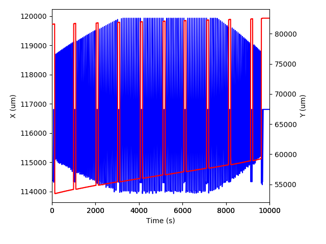
import matplotlib.pyplot as plt

# Get data
laserX = data.timeSeries('Laser_x')
laserY = data.timeSeries('Laser_y')

group = data.selectionGroup('G_NIST610')

x = [data.result(s, laserX).value() for s in group.selections()]
y = [data.result(s, laserY).value() for s in group.selections()]

plt.plot(x, y, 'o')
plt.xlabel('X (um)')
plt.ylabel('Y (um)')

plt.savefig('/Users/japetrus/Desktop/xy.png')
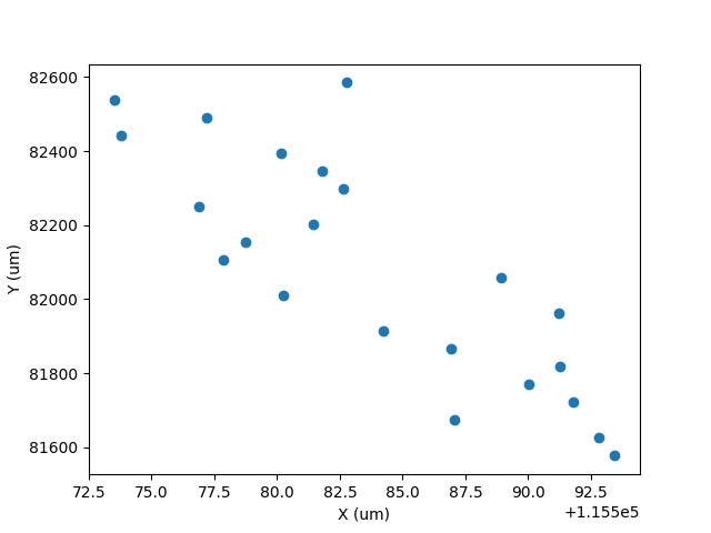
Click here to discuss.
Comparing splines - part 1
Curve fitting plays an import role in iolite's data reduction pipeline. In order to get accurate results we must have an accurate representation of how our backgrounds and sensitivities are evolving with time. iolite 3's automatic spline was very good at providing a smooth but not too smooth representation of our data. We wanted to recreate that functionality in iolite 4, but since we no longer have access to Igor Pro's fitting functions we had to go back to the drawing board.
Scanning the Igor Pro documentation regarding smoothing splines, one can discover that their implementation is based on "Smoothing by Spline Functions", Christian H. Reinsch, Numerische Mathematik 10, but it also had some iolite special sauce. Hoping to keep our splining relatively consistent from iolite 3 to 4, especially the automatic spline, this algorithm seemed like a good place to start. It turns out that this algorithm is quite popular (> 2500 citations!). One adaptation of this algorithm that also adds generalized cross validation for the automatic choice of smoothing parameter was published in "Algorithm 642: A fast procedure for calculating minimum cross-validation cubic smoothing splines", M.F. Hutchinson, Transactions on Mathematical Software 12, and it is this algorithm on which iolite 4's automatic spline is based.
Comparing with iolite 3
iolite 4 comes with the igor python module bundled so you can read data from pxp files (i.e. iolite 3) in python. We can make use of this module to extract iolite 3 spline data for comparison with iolite 4 after importing an iolite 3 pxp session into iolite 4. See below for one way of doing that.
from igor import packed
import numpy as np
import matplotlib.pyplot as plt

# Specify the group and channel to check:
group_name = 'G_NIST612'
channel_name = 'Fe57'

# Figure out which pxp was imported into iolite 4:
f = data.importedFiles()[0].filePath()
if not f.endswith('pxp'):
    raise RuntimeError('No iolite 3 experiment open?')

# Load that pxp using the igor python module:
d = packed.load(f)[1]

# Get the spline data and time for the group and channel specified for iolite 3:
splines_folder = d['root'][b'Packages'][b'iolite'][b'integration'][b'Splines']
i3spline = splines_folder[b'%b_%b'%(channel_name.encode('utf-8'), group_name.encode('utf-8'))].wave['wave']['wData']
i3t = np.copy(splines_folder[b'TimeWave_%b'%(group_name.encode('utf-8'))].wave['wave']['wData'])
i3t -= i3t[0] # Adjust the time so it starts at 0

# Get the spline data and time for the group and channel specified for iolite 4:
i4spline = data.spline(group_name, channel_name)
i4data = np.copy(i4spline.data())
i4t = np.copy(i4spline.time())
i4t -= i4t[0] # Adjust the time so it starts at 0

# Interpolate the iolite 4 data to be on the same time frame as iolite 3's spline:
i4_3t = np.interp(i3t, i4t, i4data)

# Calculate a percent difference between the two
i4_3t = 100*(i4_3t-i3spline)/i4_3t

# Plot it:
plt.clf()
plt.plot(i3t, i3spline, label='iolite 3')
plt.plot(i4t, i4data, label='iolite 4')
#plt.plot(i3t, i4_3t) # to plot percent diff instead
plt.xlim( (0, 10000) )
plt.lengend()
plt.xlabel('Time (s)')
plt.ylabel('%s - %s Spline %% difference'%(group_name, channel_name))
plt.savefig('/home/japetrus/Desktop/spline_compare.png')
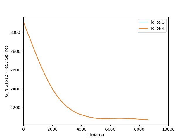
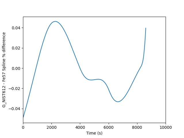
This is fine, but the two splines are almost perfectly on top of each other, so it is easier to see the difference if we plot a percent difference. This requires only a few small changes to the above script to achieve. The output looks as follows where you can see a mere 0.04 % difference between the two.
Comparing different spline types
Sometimes it is also nice to see visualize how several different spline types match up with the measured data on which they're based. The script below is one example of how you can do that.
import matplotlib.pyplot as plt
import numpy as np

# Specify the group and channel to do the comparison for:
group_name = 'G_NIST612'
channel_name = 'Fe57'

group = data.selectionGroup(group_name)

# Make a list of spline types to compare:
stypes = ['Spline_NoSmoothing', 'Spline_AutoSmooth', 'MeanMean', 'LinearFit']

# Collect the measurement data into lists:
x = [s.startTime.toMSecsSinceEpoch()/1000 for s in group.selections()]
y = [data.result(s, data.timeSeries(channel_name)).value() for s in group.selections()]
yerr = [data.result(s, data.timeSeries(channel_name)).uncertaintyAs2SE() for s in group.selections()]

# Plot the measurement data as error bars:
plt.errorbar(x, y, yerr=yerr, xerr=None, fmt='ko', label='Measurements')

# For each of the spline types, get the spline and plot it
for st in stypes:
    group.splineType = st
    s = data.spline(group_name, channel_name)
    plt.plot(s.time(), s.data(), label=st)

# Finish up with the plot:
plt.legend()
plt.xlim( np.min(x)-100, np.max(x) + 100 )
plt.ylabel('Spline for %s and %s (CPS)'%(group_name, channel_name))
plt.xlabel('Time since epoch (s)')
plt.savefig('/home/japetrus/Desktop/spline_test.png')
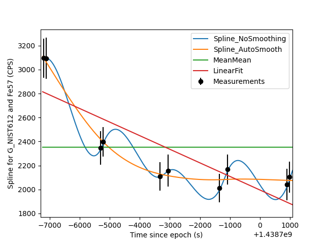
Click here to discuss.
Accessing session data from 3rd party software
In iolite 3, sessions were saved as Igor Pro "packed experiment" pxp files. This was convenient because iolite 3 was built on top of Igor Pro. The main downside to this was that Igor Pro pxp files cannot be easily read by most 3rd party software. In iolite 4, sessions are saved as files with an "io4" extension. However, this extension is just for show as the data format of the file is actually HDF5. This is super convenient because many scientific data analysis and plotting packages support the HDF5 format.
As an example, let's go through how you can load data from an iolite 4 session file into Igor Pro to be plotted.
Making Igor Pro aware of HDF
Igor Pro comes with all the tools to enable HDF interaction but it does not enable them by default. To enable Igor's HDF functionality (for Igor Pro 8 64bit, others may differ):
Go to the Help -> Show Igor Pro Folder menu item.
Go to the Help -> Show Igor Pro User Files menu item.
Navigate to "More Extensions (64-bit)/File Loaders" in the Igor Pro folder, find "HDF5-64.xop" and copy it (or make a shortcut to it).
Paste "HDF5-64.xop" in the "Igor Extensions (64-bit)" folder in the User Files folder.
Navigate to "Wavemetrics Procedures/File Input Output" in the Igor Pro folder, find "HDF5 Browser.ipf" and copy it (or make a shortcut to it).
Paste "HDF5 Browser.ipf" in the "Igor Procedures" folder in the User Files folder.
Restart Igor Pro.
That's it. You should now be able to access the HDF data browser by going to the Data -> Load Waves -> New HDF5 Browser menu item in Igor Pro.

Importing some data
When you activate the "New HDF5 Browser" menu item, you will be greeted by a dialog that looks as follows:

To start, we click the highlighted "Open HDF5 File" button and select the iolite 4 session file we want to get some data from. Once the file is loaded, you can navigate the various groups on the left and datasets on the right. Once you have found a channel you want to plot, you can select it and lick the "Load Dataset" button highlighted below.

You may need to repeat this process a few times to get all the channels you want loaded into Igor Pro. Also note that some channels use "IndexTime", which you can find in the "Special" group.
Adjusting the time
Igor and iolite handle time a bit differently. If it matters to you that the time axis is the true value, you'll want to adjust it as follows (e.g. in the Command Window - Ctrl+J or Cmd+J):
IndexTime += Date2Sec(1970, 1, 1)
Making a plot
Now that you have the channel and time data loaded, you can make a plot in the usual Igor Pro way. You can start by going to the Windows -> New Graph menu item and selecting the time as X and the channel as Y. I chose one of the final age outputs to plot and made some adjustments to the style:

Click here to discuss.
Examining Covariance and Correlation in iolite
In this example, I'll be using the gabbros dataset that you can download from here (~10 MB) but you can use this code on any data.
A quick correlation matrix as a heatmap
A correlation matrix is just a table of correlation factors comparing each input to every other input. Typically these are shown as a table of numbers, but using the python Seaborn library, we can create a heatmap that shows the correlation factor as a color to help the viewer quickly determine the which elements have some sort of linear relationship.
In this example, we'll just look at the data for a single selection (the first selection in the group 'Plag'), but you can easily extend this to all selections. I would recommend using data within selection intervals rather than all the data for a channel. It will be more specific, and won't include background counts etc.
You can copy and paste the following into a new tab in the Python Workspace to try it out. You may have to replace the whitespace at the start of the lines below the ax.set_ticklabels() and ax.set_xticklabels lines if you receive an indentation error message.
import pandas as pd
import seaborn as sns
from matplotlib import pyplot as plt

#get data for one selection
sg = data.selectionGroup("Opaq")
sel = sg.selections()[0]

df = pd.DataFrame()
#add all output channels to dataframe:
for ts in data.timeSeriesList(data.Output):
    df[ts.name] = ts.dataForSelection(sel)

corr = df.corr()
ax = sns.heatmap(
    corr,
    vmin=-1, vmax=1, center=0,
    cmap=sns.diverging_palette(20, 220, n=200),
    square=True
)
ax.set_xticklabels(
    ax.get_xticklabels(),
    rotation=45,
    horizontalalignment='right'
)

plt.show()
This should produce a nice heatmap plot that looks something like this:
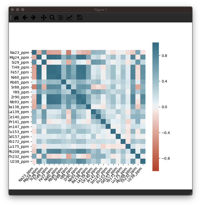
In this example dataset, there is a strong correlation between Fe, Ti and Ni, which is what we would expect for this sample (an Fe-Ti oxide). It's not necessary, but you can confirm this in the Time-Series View:
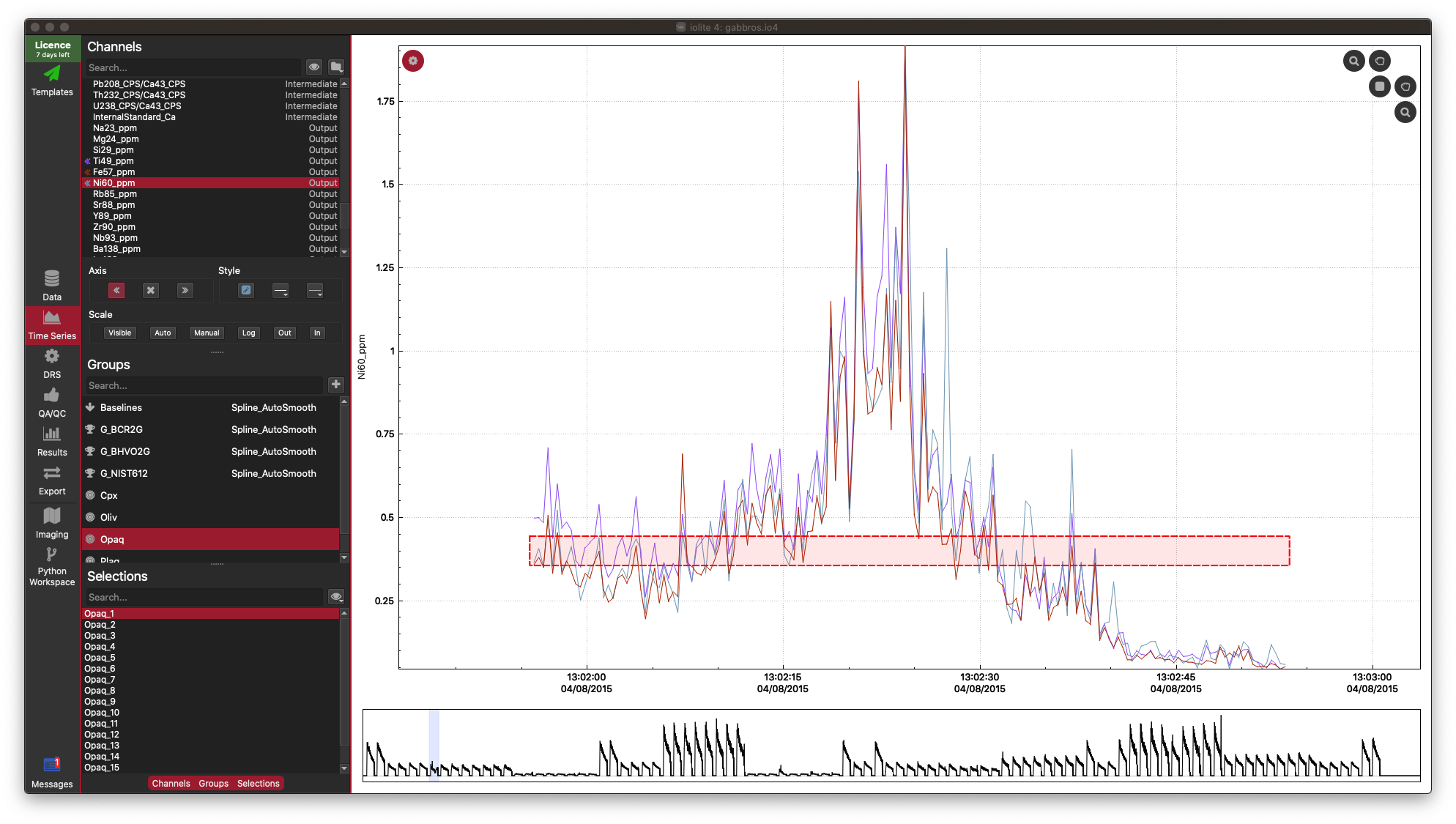
In the Time Series View, you can see that Fe (red), Ti (purple), and Ni (aqua) are very well correlated.
Correlation heatmaps are a nice simple way of looking at linear relationships between elements, but correlation coefficients don't provide information about non-linear releationships, and are exaggerated by outliers. They can also be disturbed when your data forms clusters. However, non-linear relationships are easily picked up by the human eye, and we naturally discard outliers when viewing scatterplots. So let's look at how to create a scatterplot-matrix.
Creating Scatterplot Matrices using Pandas
A scatterplot-matrix is exactly as it sounds: a matrix of scatterplots where each plot is one input plotted against another. Instead of showing a 1:1 plot along the diagonal of the matrix, we can instead show a kde (similar to a histogram) to add more information to the plot. In this example, we have many channels, and the plotting function is a little slow, so it might take a few seconds for your plot to appear.
This time we're just going to plot the first 10 channels of data.
To use this code, just copy and paste it into an empty tab in your Python Workspace:
import pandas as pd
from pandas.plotting import scatter_matrix
from matplotlib import pyplot as plt

#get data for one selection
sg = data.selectionGroup("Opaq")
sel = sg.selections()[0]

df = pd.DataFrame()
# add all output channels to dataframe... just using the first 10 channels:
for ts in data.timeSeriesList(data.Output)[:10]:
    df[ts.name] = ts.dataForSelection(sel)

sp = scatter_matrix(df, alpha = 0.2, figsize = (6, 6), diagonal = 'kde')

plt.show()
You should be able to see something like this:
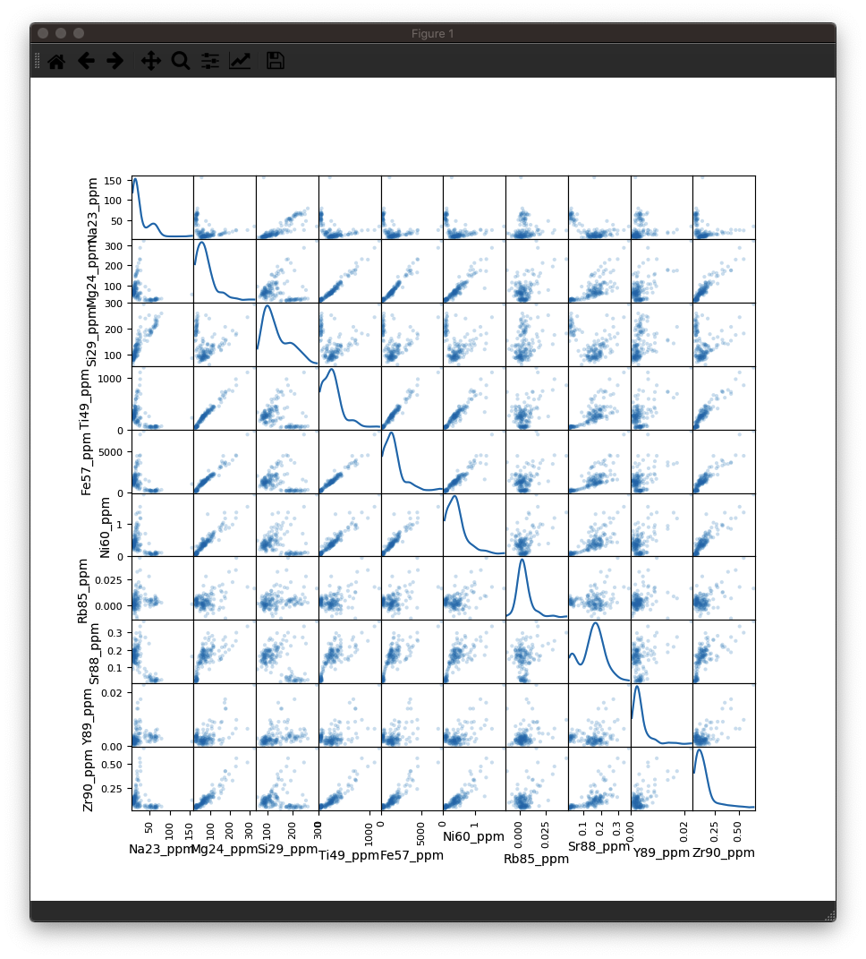
As you can see, there is a lot of information packed into an image like this, and it soon becomes crowded with more than 10 inputs. However, there is more to observe in such plots. For example even though the correlation heatmap showed Na23_ppm was not strongly correlated with other elements (with perhaps the exception of Si29_ppm), we can see in the scatterplots that perhaps there are two clusters of data when plotted against most other elements. This suggests that for this selection we may have ablated more than one phase (mineral). When we look at this selection in time-series (below), we can see that there is a low-Na, higher-Ti period followed by a higher-Na, lower-Ti interval. In this case, it may have simply been a drill through.
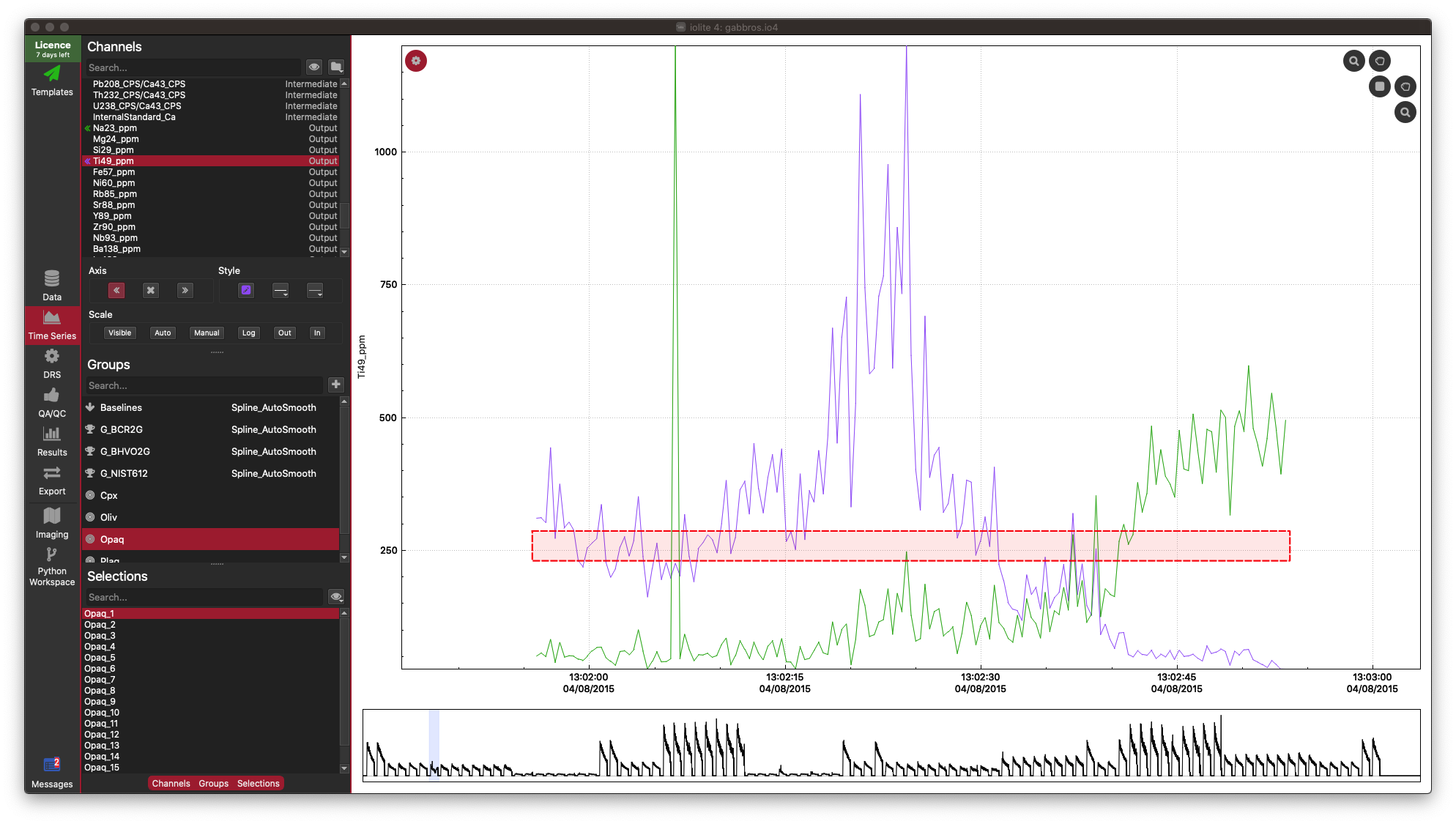
This is just a trivial example to show how to plot scatterplot matrices and correlation heatmaps in iolite. These tools can be quite helpful, especially for imaging when it is more likely that you'll be ablating different phases, tissue types etc.
If you have any questions or suggestions for improvement, please click here to discuss.
Weighted U/Ca via a simple UI plugin
A recent publication by Cogné et al. used a modified iolite 2/3 data reduction scheme to calculate 'weighted' U/Ca as part of an apatite fission track dating protocol. In this note, we will go through recreating that functionality as an iolite 4 user interface (UI) plugin.
Creating a new UI plugin
Creating a new UI plugin can be done by adding a python file to iolite's UI plugins path with appropriate meta data and required function definitions. To make this process a bit easier, you can create a new plugin from the Tools → Plugins → Create menu item. In the dialog that pops up you can set the type to UI and enter reasonable things for the other parameters.
The meta data
The first thing we need to do is define some meta data at the top of the python file. The only part that really matters is that the type is specified as UI. In doing so, we tell iolite to handle this script as a UI plugin and look for the associated functions (i.e. createUIElements below). The meta data that I wrote was as follows.
#/ Type: UI
#/ Name: WeightedUCa
#/ Description: Calculates weighted U/Ca
#/ Authors: J. Petrus
#/ References:
#/ Version: 1.0
#/ Contact: joe@iolite-software.com
Integration in iolite's interface
As mentioned above, iolite looks for a function called createUIElements in UI plugins to establish hooks in the user interface that allow a user to interact with the plugin. In this example, we'll just create a menu item that triggers the calculation by calling (a yet to be defined) run function. The way we do this is as follows.
from iolite.QtGui import QAction

def createUIElements():
    action = QAction('Calculate Weighted U/Ca')
    action.triggered.connect(run)
    ui.setAction(action)
    ui.setMenuName(['Tools'])
Calculating unweighted U/Ca
The first step in working out the weighted U/Ca is to calculate the unweighted U/Ca. The easiest way to do that is to use the U and Ca concentration channels previously calculated by a trace elements data reduction scheme. Recalling that you can get the data associated with a channel as data.timeSeries(channel_name).data() this is easily accomplished as follows.
# Create U/Ca from ppm channels
U_Ca = data.timeSeries('U238_ppm').data()/data.timeSeries('Ca43_ppm').data()
U_Ca_channel = data.createTimeSeries('U/Ca', data.Output, None, U_Ca)
Note that in the call to createTimeSeries we specify data.Output as the channel type and None as the time array. By specifying None as the time array it will default to whatever the current index time is.
Ensuring we have beam seconds
In the calculations that follow, we would like to use beam seconds and information about pit depth to work out the actual depth. One way we can do that is as follows.
try:
    bs = data.timeSeries('BeamSeconds')
except:
    bs = data.createBeamSeconds('log')
Here we have used a try-except pair to first try to get an existing beam seconds channel, and if that fails, create a beam seconds channel using the laser log. Note that the createBeamSeconds method is only available in iolite > 4.3.4.
Dialog and settings
One thing we would like to be able to do is specify a few input parameters to the calculation, such as pit depth, fission track length, and analysis duration. We can accomplish this by using QSettings and various components of QtGui as follows.
# Start by importing the necessary modules
from iolite.QtGui import QDialog, QFormLayout, QLineEdit, QDialogButtonBox
from iolite.QtCore import QSettings

# Now use QSettings to retrieve previously saved values or use defaults
settings = QSettings()
pitDepth = settings.value("WeightedUCa/pitDepth", 12.5)
trackLength = settings.value("WeightedUCa/trackLength", 8.0)
duration = settings.value("WeightedUCa/duration", 30.0)

# Construct the dialog with a QFormLayout
d = QDialog()
d.setLayout(QFormLayout())

# Add an input for depth
depthLineEdit = QLineEdit(d)
depthLineEdit.text = str(pitDepth)
d.layout().addRow("Pit depth (μm)", depthLineEdit)

# Add an input for track length
lengthLineEdit = QLineEdit(d)
lengthLineEdit.text = str(trackLength)
d.layout().addRow("Track length (μm)", lengthLineEdit)

# Add an input for duration
durLineEdit = QLineEdit(d)
durLineEdit.text = str(duration)
d.layout().addRow("Duration (s)", durLineEdit)

# Add some buttons to bottom of the dialog
bb = QDialogButtonBox(QDialogButtonBox.Ok | QDialogButtonBox.Cancel, d)
d.layout().addRow(bb)
bb.accepted.connect(d.accept)
bb.rejected.connect(d.reject)

# Run the dialog requiring a user to click ok or cancel to dismiss it
# If cancelled, return (i.e. do nothing)
if d.exec_() == QDialog.Rejected:
    return

# Get the values in the various inputs as floating point numbers
# (rather than strings) and store them in our settings
pitDepth = float(depthLineEdit.text)
settings.setValue("WeightedUCa/pitDepth", pitDepth)
trackLength = float(lengthLineEdit.text)
settings.setValue("WeightedUCa/trackLength", trackLength)
duration = float(durLineEdit.text)
settings.setValue("WeightedUCa/duration", duration)
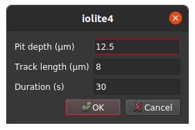
Doing the calculation
Using the appendix of the Cogné et al. publication as a reference, the weighted U/Ca can be calculated as follows.
import numpy as np
from math import pi

# Volume of a sphere
def VS(r):
    return (4/3)*pi*r**3

# Partial volume of a sphere filled to h
def PVS(r, h):
    return (1/3)*pi*h**2*(3*r - h)

def calcWtd(s, d, dur, l):
    '''
    s: selection
    d: depth
    dur: duration
    l: track length
    '''

    # Get the beam seconds and unweighted U/Ca for the specified selection
    # as numpy arrays
    sbs = data.timeSeries('BeamSeconds').dataForSelection(s)
    UCa = data.timeSeries('U/Ca').dataForSelection(s)

    x = (d/dur)*sbs # Actual depth
    dx = (d/dur)*(sbs[-1] - sbs[-2]) # Depth increment per time-slice
    weight = 2*(PVS(l, l-x) - PVS(l, l-x-dx))/VS(l)
    weight[weight<0] = 0 # Replace weights < 0 with 0 (i.e. when depth > track length)

    # Return the weighted U/Ca
    return np.sum(weight*UCa)/np.sum(weight)
Doing the calculation for all selections
Now we have the calculation in place taking 1 selection as a parameter, so we just need to iterate through the selections to calculate it for everything. One way to do that is as follows.
# Create an array of zeros matching the length of the unweighted U/Ca array
wtdUCa = np.zeros(len(U_Ca))

# Loop through groups that are RM or Sample type:
for group in data.selectionGroupList(data.ReferenceMaterial | data.Sample):
    # Loop through selections in each group:
    for s in group.selections():
        # Calculate the weighted U/Ca for this selection and replace the part
        # of the wtdUCa array corresponding to this selection with the value
        wtdUCa[U_Ca_channel.selectionIndices(s)] = calcWtd(s, pitDepth, duration, trackLength)

# Lastly, create a new channel
data.createTimeSeries('Weighted U/Ca', data.Output, None, wtdUCa)
And that's it! The newly created channel will have the weighted U/Ca and results for it can be exported along with your other data and/or viewed and manipulated in all the usual iolite ways.
Putting it all together
#/ Type: UI
#/ Name: WeightedUCa
#/ Description: Calculates weighted U/Ca
#/ Authors: J. Petrus
#/ References:
#/ Version: 1.0
#/ Contact: joe@iolite-software.com

from iolite.QtGui import QAction, QDialog, QFormLayout, QLineEdit, QDialogButtonBox
from iolite.QtCore import QSettings

import numpy as np
from math import pi

def createUIElements():
    action = QAction('Calculate Weighted U/Ca')
    action.triggered.connect(run)
    ui.setAction(action)
    ui.setMenuName(['Tools'])

def VS(r):
    return (4/3)*pi*r**3

def PVS(r, h):
    return (1/3)*pi*h**2*(3*r - h)

def calcWtd(s, d, dur, l):
    sbs = data.timeSeries('BeamSeconds').dataForSelection(s)
    UCa = data.timeSeries('U/Ca').dataForSelection(s)

    x = (d/dur)*sbs
    dx = (d/dur)*(sbs[-1] - sbs[-2])
    weight = 2*(PVS(l, l-x) - PVS(l, l-x-dx))/VS(l)
    weight[weight<0] = 0

    return np.sum(weight*UCa)/np.sum(weight)

def run():
    settings = QSettings()
    pitDepth = settings.value("WeightedUCa/pitDepth", 12.5)
    trackLength = settings.value("WeightedUCa/trackLength", 8.0)
    duration = settings.value("WeightedUCa/duration", 30.0)

    d = QDialog()
    d.setLayout(QFormLayout())

    depthLineEdit = QLineEdit(d)
    depthLineEdit.text = str(pitDepth)
    d.layout().addRow("Pit depth (μm)", depthLineEdit)

    lengthLineEdit = QLineEdit(d)
    lengthLineEdit.text = str(trackLength)
    d.layout().addRow("Track length (μm)", lengthLineEdit)

    durLineEdit = QLineEdit(d)
    durLineEdit.text = str(duration)
    d.layout().addRow("Duration (s)", durLineEdit)

    bb = QDialogButtonBox(QDialogButtonBox.Ok | QDialogButtonBox.Cancel, d)
    d.layout().addRow(bb)
    bb.accepted.connect(d.accept)
    bb.rejected.connect(d.reject)

    if d.exec_() == QDialog.Rejected:
        return

    pitDepth = float(depthLineEdit.text)
    settings.setValue("WeightedUCa/pitDepth", pitDepth)
    trackLength = float(lengthLineEdit.text)
    settings.setValue("WeightedUCa/trackLength", trackLength)
    duration = float(durLineEdit.text)
    settings.setValue("WeightedUCa/duration", duration)

    # Create U/Ca from ppm channels
    U_Ca = data.timeSeries('U238_ppm').data()/data.timeSeries('Ca43_ppm').data()
    U_Ca_channel = data.createTimeSeries('U/Ca', data.Output, None, U_Ca)

    # Make sure we have beam seconds
    try:
        bs = data.timeSeries('BeamSeconds')
    except:
        bs = data.createBeamSeconds('log')

    # Loop through selections and calculate weighted U/Ca
    wtdUCa = np.zeros(len(U_Ca))
    for group in data.selectionGroupList(data.ReferenceMaterial | data.Sample):
        for s in group.selections():
            wtdUCa[U_Ca_channel.selectionIndices(s)] = calcWtd(s, pitDepth, duration, trackLength)

    data.createTimeSeries('Weighted U/Ca', data.Output, None, wtdUCa)
Click here to discuss.
Using IsoplotR in iolite
With Kenneth Ludwig's Isoplot becoming more and more difficult to use in modern Excel (let alone on a Mac), there is increasing interest in alternatives. One alternative is Pieter Vermeesch's IsoplotR. In this note, we will have a look at one way you can use IsoplotR from directly in iolite 4.
Requirements
IsoplotR, as the name implies, reimplements much of the Isoplot functionality (and more) in the R programming language. So, the first task is getting R installed. This can be done following the recommendations for your platform and will not be covered in detail here.
The next task is getting IsoplotR installed in this R environment. With a working R installation, this should be as easy as starting the R interpreter and running:
install.packages('IsoplotR')
Of course, in iolite, we have an embedded python interpreter, but no R interpreter. So, the next task is installing the rpy2 python module. You can install this package using the procedure described in an earlier note.
If everything goes according to plan, we should now be ready to call IsoplotR functions from iolite's python interpreter!
Using IsoplotR to calculate a concordia age
As an example, we will go through compiling the required data, using IsoplotR to calculate a concordia age, and then retrieving the output.
The first thing we need to do is compile all of the measurements to feed into IsoplotR. One way we can do that is as follows:
import pandas as pd

# Choose a group
group = data.selectionGroup('Z_Plesovice')

# Compile the measurements into separate lists
r68 = [data.result(s, data.timeSeries('Final Pb206/U238')).value() for s in group.selections()]
r68s = [data.result(s, data.timeSeries('Final Pb206/U238')).uncertaintyAs2SE() for s in group.selections()]
r75 = [data.result(s, data.timeSeries('Final Pb207/U235')).value() for s in group.selections()]
r75s = [data.result(s, data.timeSeries('Final Pb207/U235')).uncertaintyAs2SE() for s in group.selections()]
rho = [data.associatedResult(s, 'rho 206Pb/238U v 207Pb/235U').value() for s in group.selections()]

# Now create a pandas data frame from those lists
df = pd.DataFrame({
    'x': r75,
    'sx': r75s,
    'y': r68,
    'sy': r68s,
    'rho': rho
})
Now we have all of our results for the 'Z_Plesovice' selection group in a pandas data frame called 'df'. The next step is to convert this into something R, and more importantly, IsoplotR can use. To do that, we'll make use of some functionality in rpy2 and IsoplotR.
from rpy2 import robjects as ro
from rpy2.robjects.packages import importr
from rpy2.robjects import pandas2ri
from rpy2.robjects.conversion import localconverter

ir = importr('IsoplotR')

# Use rpy2's functionality to convert a pandas data frame to an R data frame
with localconverter(ro.default_converter + pandas2ri.converter):
    rdf = ro.conversion.py2ri(df)

# Now use IsoplotR's functionality to convert that data frame into the format it wants
ird = ir.read_data_data_frame(rdf)
We are most of the way there at this stage! Now we just need to call a function in IsoplotR and get the output. We can do that as follows:
out = ir.concordia_age(ird)
age = out[3][0]
It is as easy as that. There are many different things output by the concordia age calculation, but the indices used (3 and 0) will be the age in Ma.
Using IsoplotR to plot the concordia age
We can also make one small change to instead plot the concordia diagram:
ir.concordia(ird, show_age=1)
This will open a window with a plot showing the measurements as well as the concordia age.
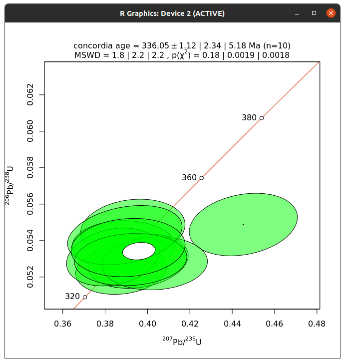
This works fine, but please note that there may be some problems with the resulting window. At least in testing this on Linux, the window cannot be closed.
Putting it all together
from rpy2 import robjects as ro
from rpy2.robjects.packages import importr
from rpy2.robjects import pandas2ri
from rpy2.robjects.conversion import localconverter

import pandas as pd

ir = importr('IsoplotR')

group = data.selectionGroup('Z_Plesovice')

r68 = [data.result(s, data.timeSeries('Final Pb206/U238')).value() for s in group.selections()]
r68s = [data.result(s, data.timeSeries('Final Pb206/U238')).uncertaintyAs2SE() for s in group.selections()]
r75 = [data.result(s, data.timeSeries('Final Pb207/U235')).value() for s in group.selections()]
r75s = [data.result(s, data.timeSeries('Final Pb207/U235')).uncertaintyAs2SE() for s in group.selections()]
rho = [data.associatedResult(s, 'rho 206Pb/238U v 207Pb/235U').value() for s in group.selections()]

df = pd.DataFrame({
    'x': r75,
    'sx': r75s,
    'y': r68,
    'sy': r68s,
    'rho': rho
})

with localconverter(ro.default_converter + pandas2ri.converter):
    rdf = ro.conversion.py2ri(df)

ird = ir.read_data_data_frame(rdf)
y = ir.concordia_age(ird)

print('Concordia age = %f'%(y[3][0]))

# Uncomment below to display concordia diagram
#ir.concordia(ird, show_age=1)
Click here to discuss.
Replacing channel data
We recently had a question about replacing values below 0 with 0 so I thought I'd write a quick note to demonstrate one way you can do that using iolite's python functionality.
Getting channel data as numpy arrays
If you have used python for some kind of scientific computing or data analysis before, you have almost certainly used or at least heard of numpy. If you're new to python, numpy is the ubiquitous python vector/matrix math library and is the foundation of countless other libraries. Naturally, we use numpy to interface iolite's c++-based channel data to python.
Getting the data and time arrays for an iolite channel in python is as easy as:
d = data.timeSeries('U238').data()
t = data.timeSeries('U238').time()
One important thing to keep in mind is that the data is shared by c++ and python/numpy, so changes made in python are automatically reflected in the c++ side and vice versa. If you do not want to modify the data you may want to make a copy of it instead:
dcopy = np.copy(d)
# or
dcopy = d.copy()
Note that much of the iolite-specific data structures and functions are accessed via a built in data object. However, there is nothing preventing you from replacing that by doing something like data = data.timeSeries('U238').data(). If you were to do that, you would no longer be able to access iolite's data and might encounter some difficult to decipher errors!
Replacing values matching some criteria
Numpy is extremely powerful and simple to use. Supposing you want to replace values less than 0 with 0, this can be accomplished in one simple statement d[d < 0] = 0. So, if we want to replace data less than 0 for all input channels we can do this with a very simple script:
for c in data.timeSeriesList(data.Input):
    c.data()[c.data() < 0] = 0
Note that we can also do this for all channels by omitting the data.Input or we could combine channel types, e.g. data.Intermediate | data.Output.
There is only one thing left to do -- since we have changed the channel data, we should tell iolite that the data has changed and update our results.
data.updateResults() # This will update all results (and update things in the results view)
data.emitDataChanged() # This will cause the time series view to replot the data
data.activeSelectionGroup().changed.emit() # This will cause splines and selections to be replotted
Technically, the last line will cause an error if there is no active selection group (AttributeError: 'NoneType' object has no attribute 'changed'). This can be safely ignored, or if you don't want to see it, you could either check if data.activeSelectionGroup() is None or wrap it in a try/except.
Putting it all together
for c in data.timeSeriesList(data.Input):
    c.data()[c.data() < 0] = 0

data.updateResults()
data.emitDataChanged()
data.activeSelectionGroup().changed.emit()
And that's it!
Click here to discuss.
Coverting ppm channels to weight % oxide
One question that came up recently was how to get the results in weight percent oxide rather than ppm. In this note, we'll go through one way you can do that using iolite's python functionality.
Getting element data and oxide-to-element factors
We have a mini database of element/isotope data available in iolite that can be accessed from python via the data.elements dictionary. For example:
data.elements['Si']
{
    'CI': 106500.0,
    'MORB': 236000.0,
    'MUQ': 315678.758,
    'atomicNumber': 14,
    'atomicRadius': 132.0,
    'atomicWeight': 28.085,
    'block': 'p',
    'boilingPoint': 2628.0,
    'density': 2.33,
    'electronAffinity': 1.3895211,
    'geochemicalClass': 'major',
    'goldschmidtClass': 'lithophile',
    'group': 14,
    'ionizationEnergies': (8.151683, 16.345845, 33.493, 45.14179, 166.767, 205.267, 246.32, 303.66, 351.1, 401.38, 476.18, 523.415, 2437.65804, 2673.1774),
    'isotopes': (
        {
            'abundance': 0.92191,
            'mass': 27.976926535,
            'massNumber': 28
        },
        {
            'abundance': 0.04699,
            'mass': 28.976494665,
            'massNumber': 29
        },
        {
            'abundance': 0.0311,
            'mass': 29.97377001,
            'massNumber': 30
        }),
    'meltingPoint': 1683.0,
    'name': 'Silicon',
    'period': 3,
    'series': 5,
    'symbol': 'Si'
}
This data can be useful for a variety of tasks, but in this instance we are interested in using it to get atomic weights so we can calculate a conversion factor between element and oxide forms. We could do this as follows:
wSi = data.elements['Si']['atomicWeight']
wO = data.elements['O']['atomicWeight']
fSiO2 = (wSi + 2*wO)/wSi
# fSiO2 = 2.1393...
Or more conveniently, you can get this factor using a built in function:
fSiO2 = data.oxideToElementFactor('SiO2')
# fSiO2 = 2.1393...
Calculating major elements as weight % oxide
Equipped with these conversion factors, we can now calculate weight % oxide channels from our existing ppm outputs from the trace elements data reduction scheme as follows:
# Create a dict indicating the oxide formula to be used for each element
formulae = {
    'Si': 'SiO2',
    'Al': 'Al2O3',
    'Ti': 'TiO2',
    'Fe': 'Fe2O3',
    'Mn': 'MnO',
    'Mg': 'MgO',
    'Ca': 'CaO',
    'Na': 'Na2O',
    'K': 'K2O',
    'P': 'P2O5'
}

# Iterate through the elements in our dict
for el in formulae:
    # Iterate through output channels matching the current element
    # (note: there may be no matches, and that is ok)
    for c in data.timeSeriesList(data.Output, {'Element': el}):
        # Get the conversion factor for this element
        f = data.oxideToElementFactor(formulae[el])
        # Compose a string for the name of our new channel
        name = '%s%s_wt_pct_oxide'%(c.property('Element'), c.property('Mass'))
        # Create the new channel using the above info
        data.createTimeSeries(name, data.Output, None, c.data()*f/1e4)
And that's it!
Click here to discuss.
The Non-Linearity of the Age Equation and when you might notice it
"Why is the mean age calculated by iolite different to the age calculated from the mean ratio?"
This post will most likely be too simple for the more math-literate, but I'm breaking it down for those like myself that enjoy seeing these sort of concepts explained in detail. I have included a spreadsheet showing all the calculations detailed in this note that you can download from here.
If you are more math-literate, or would like a more general explanation of this effect, I recommend reading the Wikipedia entry on the Jensen's Inequality.
Lets use 207Pb/235U ratios/ages for our example, but the same applies to other ratio/ages. In the question above, the "age calculated by iolite" refers to the mean of the Final 207Pb/235U age, and is asking why this is different to the age you might calculate from the mean of the Final 207Pb/235U channel. This is due to the non-linearity of the age calculation. Just to remind you, here is the equation for calculating an age from a 207Pb/235U ratio (the equation for 206Pb/238U is very similar but uses a different constant):
$$text{age (Ma)} = frac{ln(frac{207}{235} +1)}{0.00098485}$$
the natural log part is quite important, because that tells us that the equation is non-linear. We can demonstrate that with a simple example. I'm going to take one of the selections from our U-Pb example dataset DRO4.io4 that can be downloaded from here. In particular, I've picked the third selection of Temora 2, but any selection would have done. I exported the Final 207Pb/235U and Final 207Pb/235U age values for the entire selection as a time series (so that I could see each value rather than just the mean for each channel). You can do this yourself in iolite v4 by using export settings shown below:

If you open the resulting Excel file, you'll see a worksheet for each selection in the Z_Temora2 group. I've already created a spreadsheet showing the calculations described in this Note, and removed the other unused worksheets, that you can download from here and check through to satisfy yourself.
Now if we calculate the mean of the Final 207Pb/235U ratios in our spreadsheet, we get a value of 0.503. If we were to use the age equation above, that would give us an age of about 413 Ma which pretty close to the accepted age of Temora 2 – 417 Ma. However, if we calculate the mean of the Final 207Pb/235U age values, we get a value of 409 Ma: the ages are not the same. This is the crux of the question at the top. Why aren't these values the same?
The first thing we could look at is the effect of varying our ratios. Let's add 20% to the mean ratio value (0.503) and calculate an age from these two new ratios:
Offset |
Ratio |
Calculated Age (Ma) |
Difference (%) |
|---|---|---|---|
-20% |
0.400 |
342 |
-17% |
+20% |
0.600 |
477 |
16% |
In this table, Difference (%) is the difference between the newly calculated age and the age from the mean ratio (0.503) of 413 Ma. So you can see that if we have a value 20% lower than the mean ratio, it will result in a 17% lower age, and if we have a value 20% higher, our calculated age increases by 16%. Let's exaggerate this a little further, and increase our differences to 50%:
Offset |
Ratio |
Calculated Age (Ma) |
Difference (%) |
|---|---|---|---|
-50% |
0.250 |
227 |
-45% |
+50% |
0.751 |
569 |
38% |
So, here we can see the effect even more: the lower ratio has moved the calculated age down 45%, but the higher ratio has only moved the calculated age up by 38%.
Hopefully this helps demonstrate that lower ratios pull down the calculated age more than higher ratios pull the calculated age up. And 50% isn't even that abnormal when talking about the variation we might see in Final 207Pb/235U ratios: even our example Temora 2 data vary by 67% (2 RSD).
And just to show that this isn't related to the distribution of ratios in our example dataset, let's look at a perfectly normally distributed set of ratios# with the same mean (0.503) and standard deviation (0.169) (see the spreadsheet linked above for the ratio values). If we put each of those ratios into the age equation, we end up with a negativley-skewed group of ages, because of the non-linearity of the age equation.

We have a skew to the negative side of our distribution of ages, even though we had a normal (gaussian) distribution going into the age equation. And this is why if we calculate the mean of these ages we get a different value to if we calculated an age from the mean ratio.
So, which value to use? We recommend that you use the mean ratio, and calculate an age from this. The ages that iolite shows are more to help you understand your data and to provide context, rather than actually providing an age estimate.
If you have any questions about the above, please join the discussion here.
#The values in the spreadsheet are not perfectly normally distributed, because they are a random subset of 1000 values from a normal distribution, but they are a good approximation. The values you see will likely not quite match the same values I see because Excel will create a new sample of 1000 values when you open the spreadsheet, but the principle is the same.
About masks in iolite
Masks have been part of iolite since the early days, but we still regularly get questions about them. In this note, we will take a look at what a mask is and why you might want to use one, the ways you can make one, and what it looks like when things go right (and wrong).
What is a mask
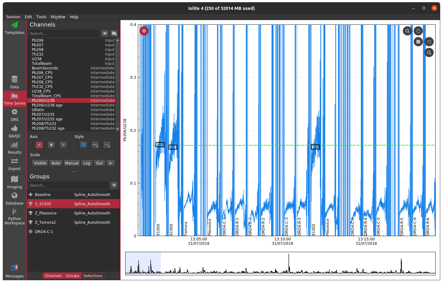
Often when working with mass spectrometry data there are intervals in the time-resolved signals that don't correspond to a sample being analyzed. In these intervals, calculated channels, such as ratios, will sometimes behave erratically making it difficult to see the part of the signal that corresponds to your sample. For example, see below where I have not used a mask and am plotting the time-resolved 206Pb/238U for a series of zircon analyses.
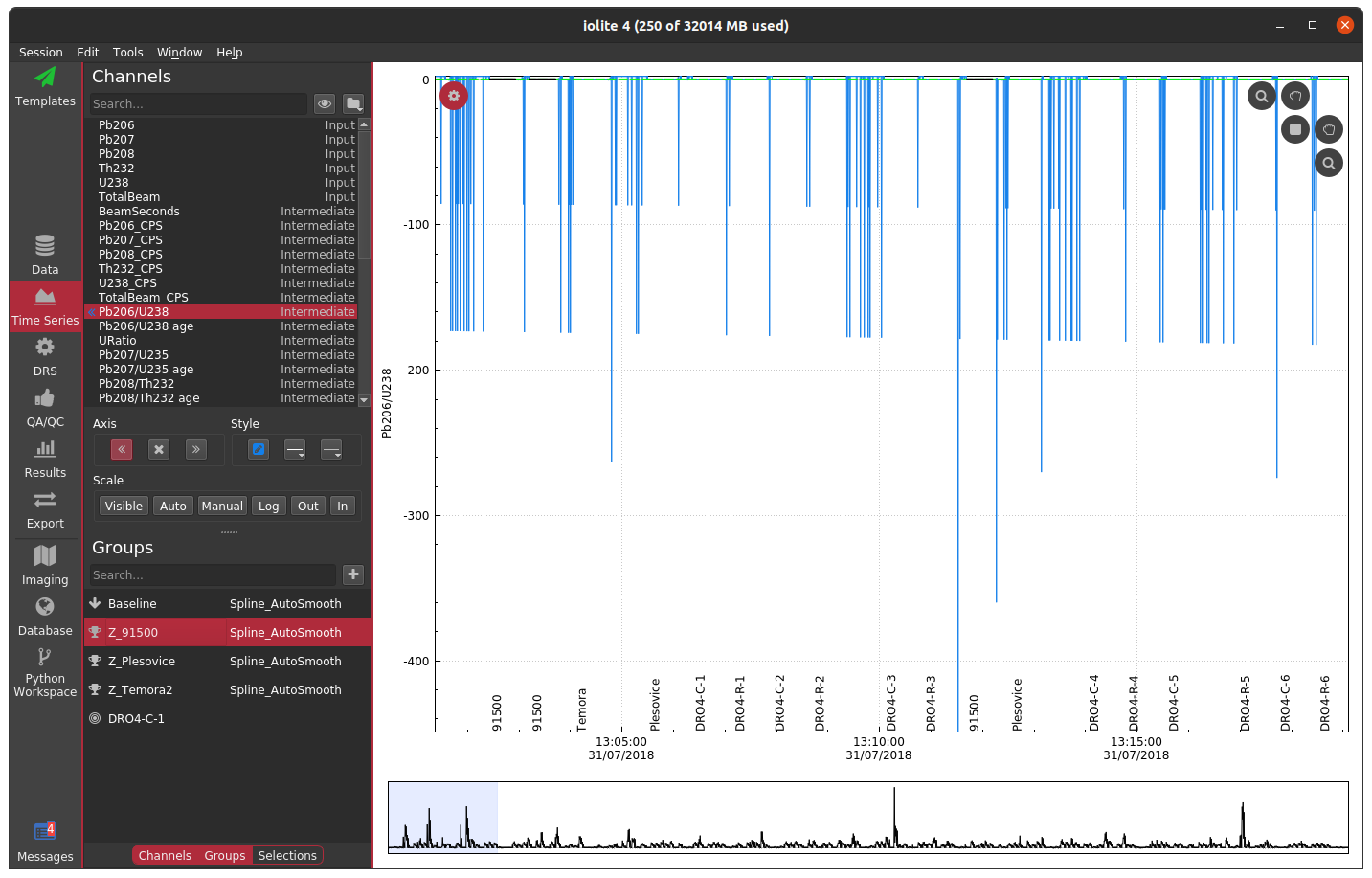
In this plot, the 91500 zircon analyses are relatively close to 0 and are relatively invariant, but since we have not applied a mask, the background regions for the ratio are strange and confuse the auto scaling. For most data reduction schemes, the backgrounds of input channels are removed (thus bringing them close to 0) and therefore calculating things like ratios is especially problematic due to dividing by very small numbers. In the above example, apparently one of the input channels' baseline subtraction resulted in the data being slightly below zero, which caused the ratio in the background to be large and negative. We could, of course, just zoom in on the relevant data as below.
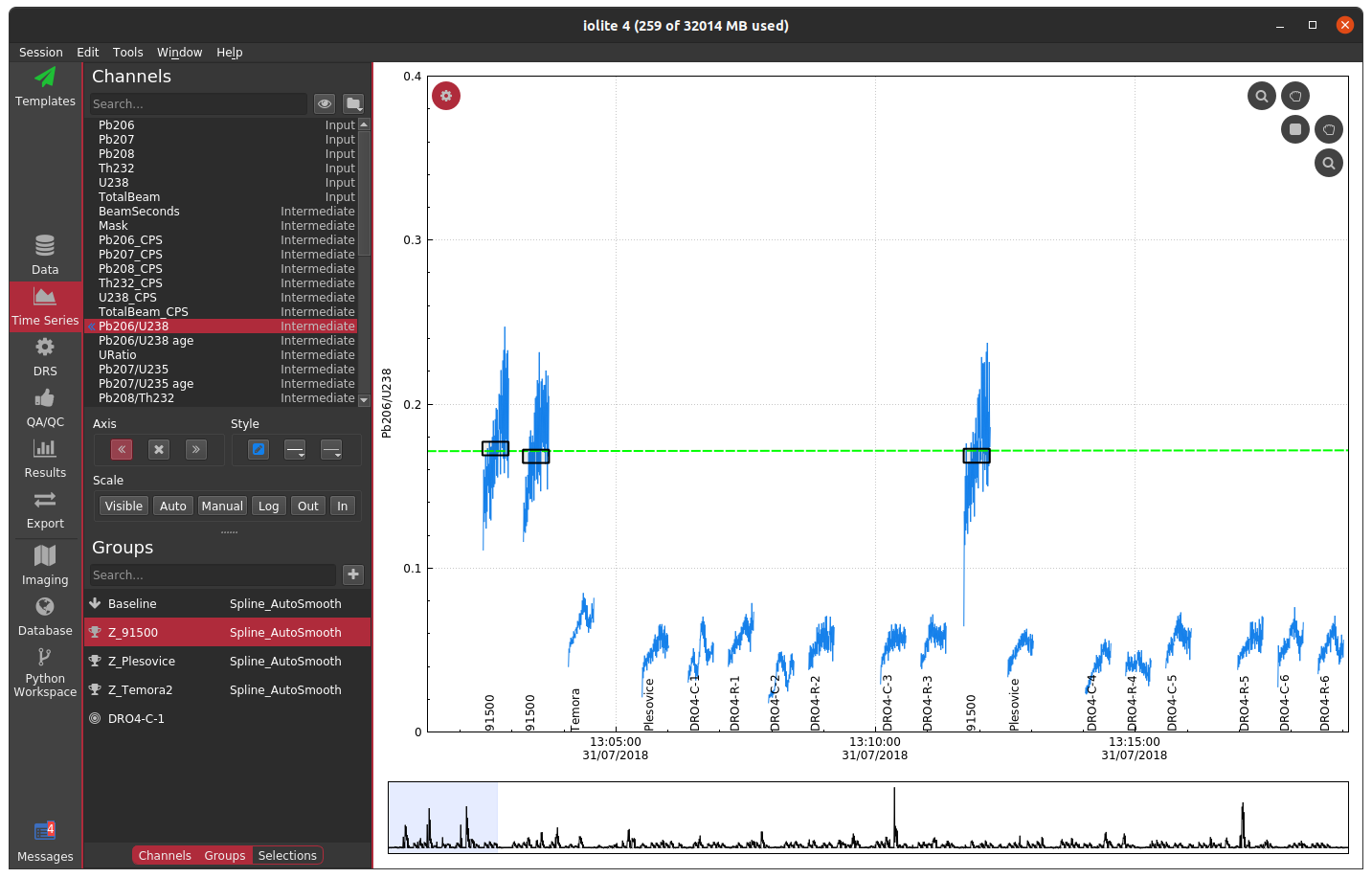
However, this is a bit unsightly and makes it difficult to see trends in the time-resolved data. A more elegant solution is to mask (i.e. hide) parts of the channels that we don't want to see. In terms of the math happening behind the scenes this is equivalent to multiplying a channel's data by an array with ones where we want to see data and nans where we don't. The mask, however it is determined, is typically applied to all calculated channels (i.e. intermediates and outputs).
It is also worth mentioning that data that have been masked will not contribute to a result. In other words, if a selection extends into masked data, the masked data do not figure into the mean, uncertainty, etc.
How to create a mask
There are two ways commonly used to create a mask in iolite. The preferred method is to use a laser log. From the laser log we know when the laser is firing and therefore know when to expect useful signals. We can use this information to construct a mask that will block out all other parts of the data in calculated channels. You can see the effect of using the laser log to construct a mask below where we no longer see the chaos between samples and can now focus on individual and long term trends.
If you do not have a laser log, you can alternatively construct a mask by using an input channel and cutoff threshold. The best channel to select and specific value to use ultimately depends on the nature of your data and which channels you have analyzed. In this zircon dataset, if I were to choose U238 and a cutoff of 500 CPS, the masked data looks as below.

If you compare the two carefully, you can notice that the cutoff used probably left a bit too much signal at the beginning and end of each spot. You could try fiddling with the channel or cutoff values to fix the issue, or you can opt to trim the mask by a configurable number of seconds at the beginning and end of each change. If we were to select a trim of 2 seconds, you get the following.
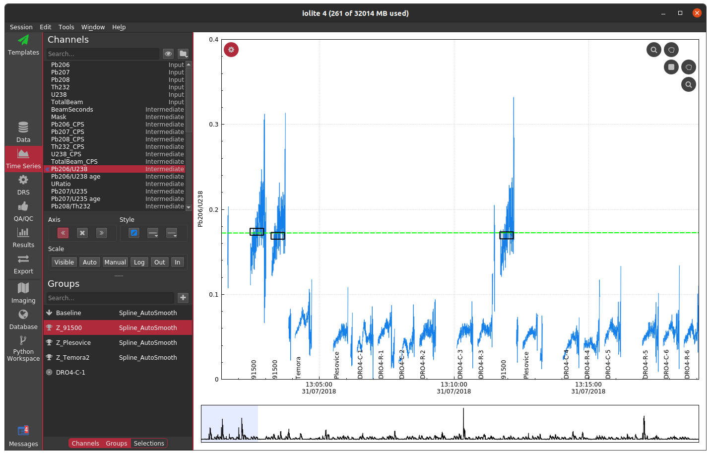
Note that the ends in particular still look erratic. The reason for this is that there are cleaning pulses between analyses that cause the U238 signal to spike and therefore the mask does not apply there. Examples like this demonstrate why a laser log is preferred -- they are more accurate and take the guess work out of the process.
When things go wrong
Of course, there are a variety of ways things can go wrong. A few examples of what to watch out for are shown below.
Laser log not aligned properly
If the laser log is not aligned to the data properly, you can end up with a mask that masks part of the good signal and doesn't mask part of the baseline (or worse), as shown below.
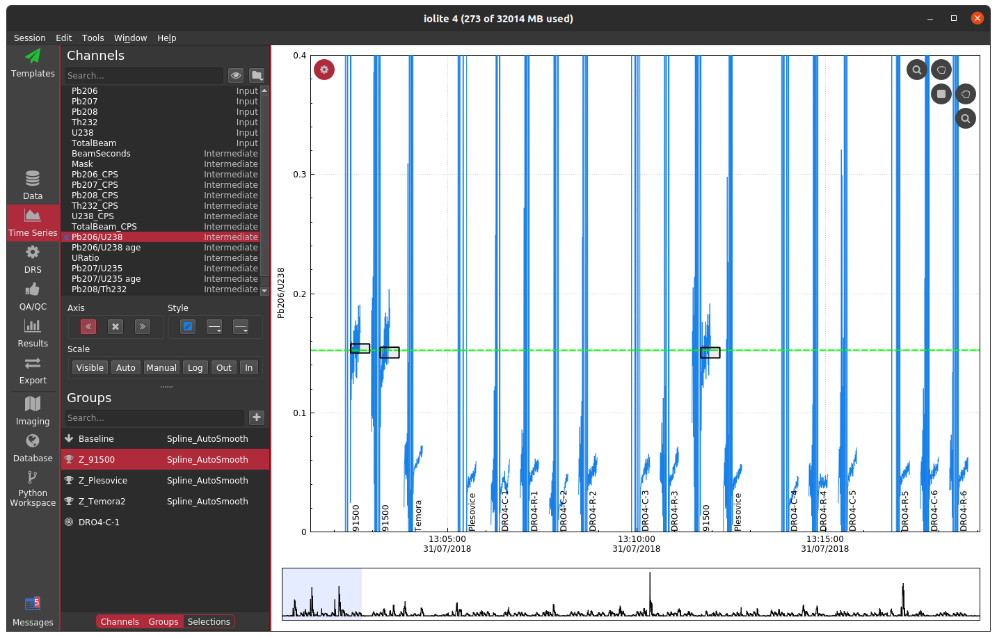
For U-Pb datasets, a misaligned laser log will also be evident in the down-hole fractionation plots if you are using the laser log for the beam seconds method.
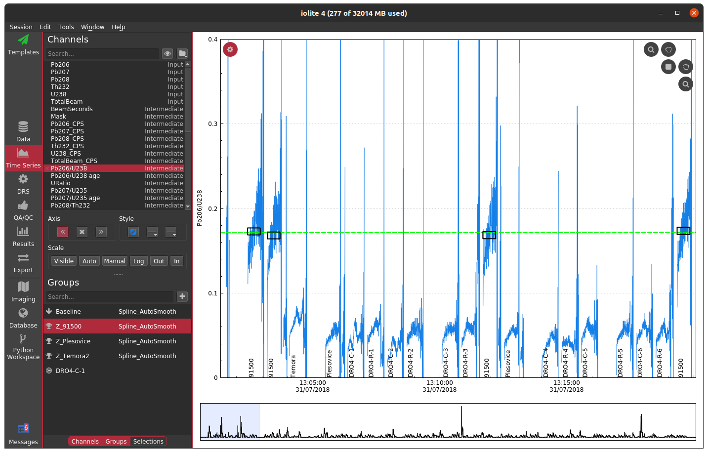
Cutoff too low
If you specify a cutoff that is too low, you can end up with something that looks like no mask at all (e.g. as above), or some intermediate.
Cutoff too high
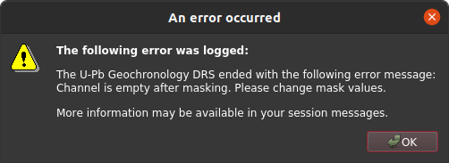
If you specify a cutoff that is too high, you can end up with all of the data masked, which may lead to other complications and/or errors depending on which data reduction scheme is in use.
Channel not consistent
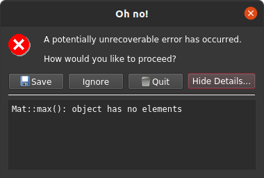
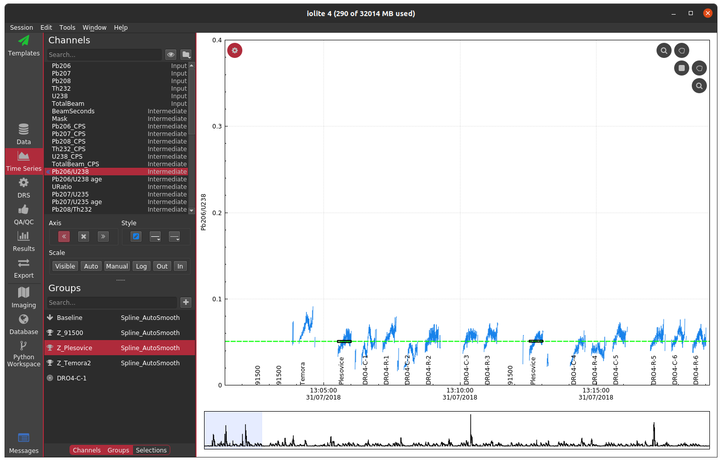
It is also possible to specify a channel and value cutoff combo that totally masks some analyses and not others. For example, in this zircon dataset it is possible to completely mask the relatively low U 91500 zircon analyses while leaving the others alone by using an intermediate U238 cutoff. If we were to do that and select 91500 as our reference material, this would produce an error as below because the data reduction scheme cannot find any data to do the correction with.
If you were to use a different reference material with same mask configuration you would find something as below, where the data corresponding to 91500 appear blank.
Thank you for reading! Click here to discuss.
Pb concentration calculations and TotalPb_ppm
For most samples, these values would be within error of one another, with 204Pb_ppm being the least precise (due to low counts) and 208Pb_ppm or TotalPb_ppm being the most precise (due to having the most counts). This is assuming that you have "normal" Pb isotopic abundances in your sample. By normal here, I mean that if you're using a NIST glass for calibration, your sample also has roughly similar Pb isotopic abundances. In case you're not familiar with the isotopic make up of modern common Pb, typical isotopic abundances are shown in Table 1.
204Pb |
206Pb |
207Pb |
208Pb |
|---|---|---|---|
1.4% |
24.1% |
22.1% |
52.4% |
If you use, for example, NIST610 to calibrate zircon analyses you may see significantly different values for each of the Pb_ppm channels. Just as an example, below are some concentrations from a randomly selected zircon calibrated with NIST610.
Pb204_ppm |
Pb206_ppm |
Pb207_ppm |
Pb208_ppm |
TotalPb_ppm |
|---|---|---|---|---|
0.70 |
22.45 |
1.16 |
1.88 |
6.70 |
Pb concentrations in this example zircon vary from 22 ppm to less than 1 ppm. So, what is going on? Which is the "correct" concentration?
Well, zircons quite regularly have very different Pb isotopic abundances than common Pb. If you've measured all four Pb isotopes (or with only very slighly less precision 206Pb, 207Pb and 208Pb), you can calculate the isotopic abundance of each isotope by ratioing the baseline subtracted counts for each channel to the baseline subtracted TotalPb counts. Here are those values for our example zircon (Table 3) along with the calculated isotopic abundances (Table 4).
Pb204_CPS |
Pb206_CPS |
Pb207_CPS |
Pb208_CPS |
TotalPb_CPS |
|---|---|---|---|---|
10.40 |
5683.54 |
265.94 |
1042.94 |
7004.60 |
204Pb |
206Pb |
207Pb |
208Pb |
TotalPb |
|---|---|---|---|---|
0% |
81% |
4% |
15% |
100% |
This is a rough calculation of isotopic abundance (it does not take into account mass bias), but it is probably sufficiently precise for trace element calculations such as this. You can see that 206Pb in this example comprises over 80% of total Pb, compared to ~24% in normal Pb.
How does our concentration calculation take this into account?
Well, normally we assume that our sample and calibration material have the same isotopic composition, and so we slightly simplify the concentration calculation. Here's a simplified version of the Longerich et al. equation, where I've left out the internal standard part (it's not important for this discussion):
$$text{[Pb]} = frac{CPS{samp}}{CPS{RefMat}}[Pb]_{RefMat} $$
Where [Pb] is the concentration of Pb in the sample, CPSsamp is the baseline subtracted counts per second for the sample, CPSRefMat is the baseline subtracted counts per second for the Reference Material, and [Pb]RefMat is the concentration of Pb in the Reference Material.
If we were to include the isotopic composition of the sample and reference material, and use for example 206Pb as our channel of interest, the equation would actually look like this:
$$text{[Pb]} = frac{CPS{samp} / [206Pb]{samp}} {CPS{RefMat} / [206Pb]{RefMat}}[Pb]_{RefMat} $$
Where [206Pb]samp and [206Pb]RefMat is the isotopic abundance of 206Pb in our sample and reference material, respectively. If our sample and reference material have the same isotopic composition, [206Pb]samp and [206Pb]RefMat will be the same value and can be simplified from the equation.
We can see the effect of using the correct isotopic abundance for our example zircon by multiplying the concentrations in Table 2 by the appropriate normal Pb isotope abundance and dividing by the calculated isotope abundance for our sample. For example, the corrected 206Pb concentration would be calculated by:
$$[Pb]_{corr} = frac {0.24[Pb]} {0.81} $$ $$ = frac {0.24(22.45)} {0.81} $$ $$ = 6.7 ppm $$
If we repeat the same process for the other Pb isotopes in our example, using the calculated isotopic abundances from Table 4 and the common Pb isotopic abundances in Table 1, we get the following corrected concentrations:
Pb204_ppm |
Pb206_ppm |
Pb207_ppm |
Pb208_ppm |
|---|---|---|---|
6.56 |
6.67 |
6.75 |
6.63 |
You can see that they all come out approximately equivalent to the original TotalPb concentration reported in Table 2 (6.7 ppm).
So, to answer the original question: which ppm result is the 'correct' one? Well, in this case where our sample does not have the same isotopic composition as our reference material, **TotalPb gives us the best estimate of the Pb concentation in our sample**.
If you have any questions or comments about this Note, you can discuss it here.
Synchronizing individual laser log samples
Laser logs can save a lot of time when setting up selections in iolite. Rather than painstakingly reviewing each bit of data and assigning it to a selection/group, the time stamps in a laser log and the analysis annotations can be matched up with mass spec data to automate this process. Usually this works great. However, there are certain combinations of instruments that just cannot seem to agree on the timing, and when this happens it can be very frustrating as what should take seconds is now taking minutes or even hours!
When a laser log is synchronized in iolite using the normal procedure (i.e. via the import log button and subsequent dialog), the laser log in its entirety is synchronized with the data using an algorithm similar to the one below. That means if the laser computer and mass spec computer do not agree on the timing, the two may be not always be in sync, and how they differ may not be predictable. This results in automatic selections starting/ending before/after they should and, more importantly, inaccurate and/or imprecise results without manual intervention. An example is shown below where the laser log has been optimally synchronized with the data, but certain analyses do not line up.
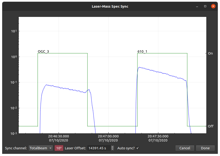
Synchronizing two signals
The task of synchronizing the laser log and the mass spec data boils down to working out the cross-correlation between the two. Usually, the laser log is represented by a square wave with 'up' and 'down' events corresponding to the laser 'on' and 'off' events recorded in the laser log, and the mass spec data is represented by the TotalBeam (sum of all input data).
There are, of course, many ways to accomplish this task in practice, one of which is included below (copied from here) and is very similar to the C++-based implementation used internally by iolite. This approach employs numpy's speedy fast Fourier transform (fft) routines and some fancy math to work out the time offset between the two signals much faster than a more verbose and non-mathematician-readable implementation (e.g. using numpy's correlate function).
import numpy as np
from numpy.fft import fft, ifft, fft2, ifft2, fftshift

def cross_correlation_using_fft(x, y):
    f1 = fft(x)
    f2 = fft(np.flipud(y))
    cc = np.real(ifft(f1 * f2))
    return fftshift(cc)

# shift < 0 means that y starts 'shift' time steps before x
# shift > 0 means that y starts 'shift' time steps after x
def compute_shift(x, y):
    assert len(x) == len(y)
    c = cross_correlation_using_fft(x, y)
    assert len(c) == len(x)
    zero_index = int(len(x) / 2) - 1
    shift = zero_index - np.argmax(c)
    return shift
For those interested in experimenting with synchronization in iolite, the above bit of python code is a good starting point. If instead you do not care about the synchronization details, but just want to get it done, you can use a helper function included as part of iolite's python API:
# with:
# x1, y1 = the time, data arrays of the first signal
# x2, y2 = the time, data arrays of the second signal
shift = data.timeOffset(x1, y1, x2, y2)
Getting and manipulating the required data
iolite's python API (introduced here and mostly documented here) provides everything we need to get the required data, synchronize, and update the laser log samples. Note: setting laser log sample start/end times via python is only supported in iolite v.4.3.10+.
Channel time and data can be access as:
t = data.timeSeries('TotalBeam').time()
# Don't do this:
# data = data.timeSeries('TotalBeam').data()
# because you'll overwrite the interface to iolite's data
d = data.timeSeries('TotalBeam').data()
Laser log samples can be accessed and manipulated from iolite's python API as follows:
samples = data.laserLogSamples() # a list of SampleMetadataPyInterface objects

st = samples[0].startTime() # start time of first sample as QDateTime type
et = samples[-1].endTime() # end time of last sample as QDateTime type

samples[0].setStartTime(st.addMSecs(5e3)) # set start time to 5 seconds later
samples[0].setEndTime(st.addMSecs(-5e3)) # set end time to 5 seconds earlier
The methods available for QDateTime objects can be found here.
Synchronizing individual laser log samples
Putting it all together, we can optimize the synchronization of each individual laser log sample locally using a script as follows.
import numpy as np

tb = data.timeSeries('TotalBeam')
sg = data.createSelectionGroup('LocalAdjustTemp', data.Sample)
ts = np.median(np.diff(tb.time()))
n = int(round(10/ts)) # 10 = number of seconds to search around log sample

for i, lls in enumerate(data.laserLogSamples()):
    sel = data.createSelection(sg, lls.startTime(), lls.endTime(), 'Temp')
    si = tb.selectionIndices(sel)
    try:
        da = tb.data()[si[0]-n:si[-1]+n] # Take n points before or after sample
        lla = np.pad(np.ones(si[-1] - si[0]), (n, n), 'constant', constant_values=(0, 0))
        offset = data.timeOffset(np.arange(len(da)), da, np.arange(len(lla)), lla)
    except Exception as e:
        print('problem for %i, %s'%(i, e))
        continue

    print('%i = %i, %f s, len(da) = %i, len(lla) = %i'%(i, offset, offset*ts, len(da), len(lla)))
    lls.setStartTime(lls.startTime().addMSecs(offset*ts*1000))
    lls.setEndTime(lls.endTime().addMSecs(offset*ts*1000))

data.removeSelectionGroup('LocalAdjustTemp')
Which, for the problem illustrated at the beginning of this note for OGC-3, produces an adjusted laser log sample as shown below. New selections created from the laser log samples will now have improved synchronization.
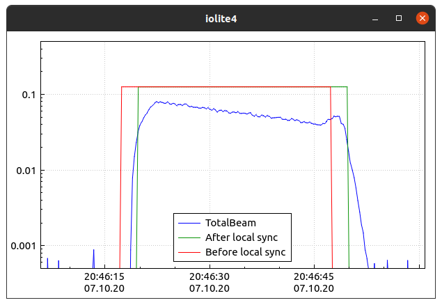
And that's it!
Click here to discuss.
Inserting Timestamps into Old Agilent Files
Using image logs in iolite
One handy feature that was slipped into iolite a while ago without much publicity is the ability to visualize "ImageLog" images in the time series view. Image logs are just what they sound like: an image captured by the laser ablation control software before and/or after each analysis. Starting with iolite v4.3.10, this feature allows you to see an image of the spot associated with the active selection in iolite's time series view, which can be very useful in evaluating whether certain elements might be from cracks, mixed targets, etc.
How it works
When you import a laser log, iolite will look for a subfolder within the folder containing the laser log file that has a matching "ImageLog" name. For example, if the log file was "My Important Work_log_20210603_120000.csv" then the corresponding ImageLog folder should be "My Important Work_ImageLog_20210603_120000". If an ImageLog folder is found, the sample names found in the laser log are matched to png image files found in the ImageLog folder, and that bit of metadata (i.e. the image file path) is stored with the imported laser log samples. Now, when a selection is made from a laser log sample in iolite, that information is copied over to the selection as an "Image" property. Finally, when the active selection details popup is activated in the time series view (by pressing the 'a' key), the image file associated with that selection is displayed along with the other details. A cross hair is also drawn on the image to help identify which pit the selection corresponds to. Depending on the magnification of the image captured, you may need want to adjust the zoom of the displayed image -- this can be done via a right-click context menu.
In action
When image log files are found and assoicated properly with selections, you will be able to see an "Image" property for each selection as shown below.
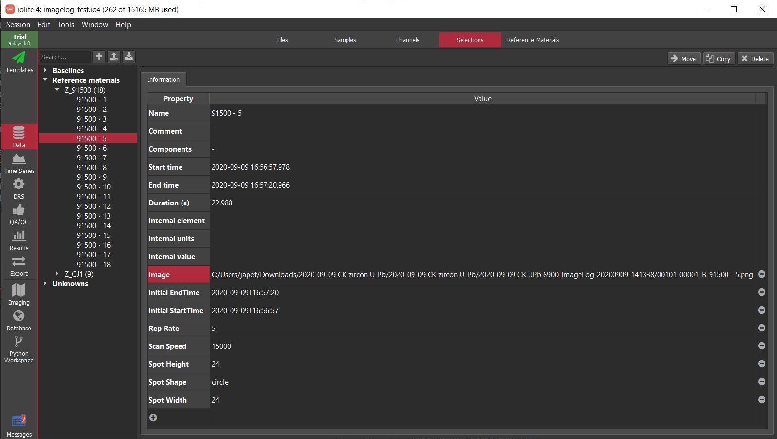
Then, when you're in iolite's time series view you can press the 'a' key with an active selection to see the image in the details popup.
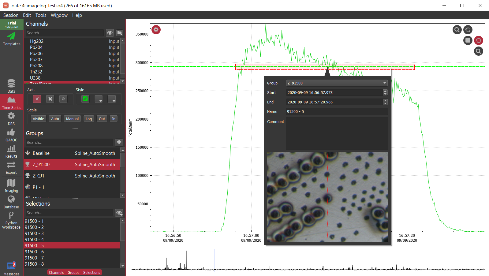
Note that if you move the image log folder after import the log file and creating selections this feature will no longer work.
If you have any questions, comments or suggestions about this Note, you can discuss it here.
About updating resources
You may have noticed a dialog that looks as below when you run iolite for the first time after updating.
The reason you are seeing this dialog is that a variety of files are included with iolite but live outside the iolite folder and may be modified by users. This poses a problem when updating iolite: we may have modified the files for the new release but you may have modified them yourself (and with good reason) locally. We do not wish to upset people by overwriting their changes, so we keep track of the *hashes* of these files as they were when putting out releases. If you have not modified any of the files yourself (i.e. their current hash on disk matches one of our releases) then we will update the file automatically. If you have modified the file (i.e. their current hash on disk does not match one of our releases) then you will see the above dialog asking you what you would like to do.
In the example shown above, I have modified the G_NIST610 reference material file and the iolite_helpers.py script that is used for fitting, concordia/discordia ages, etc. All of the checked items in the list will be updated to our latest version of that file. Unchecked items will not be updated. If you click cancel no files will be modified, but you will be prompted again next time you run iolite.
If you have any questions, comments or suggestions about this Note, you can discuss it here.
Using a polygonal ROI as a clipping mask
When acquiring images, it is fairly common that more than just the target is ablated and analyzed. For example, maybe you want to be sure that you get the material boundaries or perhaps you are not exactly sure where the boundaries are, so you setup your sequence to cover a broader area. In doing so, a potential problem arises if the material ablated beyond your target is highly variable or orders of magnitude different concentration -- making it unsightly and/or difficult to scale such that you can see the detail of your actual target.
In previous versions of iolite 4, you could setup a mask filter with channel criteria to select only the relevant part of the data. Depending on the nature of the sample, figuring out which criteria to use to select the area of interest can be tricky (or impossible). To get around this problem, we have just added (to v4.4.9) the ability to use a polygonal region of interest (ROI) as a clipping filter. Read on to see how!
How to...
It is fairly straight-forward. First, you create a polygonal ROI covering the area of the image that you want to remain visible. You can do that by clicking the inspect button in the top right corner to expose the inspection panel. In that panel, you can go to the Region of interest tab and click the Add button. Now you can place a series of vertices for the ROI by clicking on an image and double clicking to complete the polygon. An example is shown below.
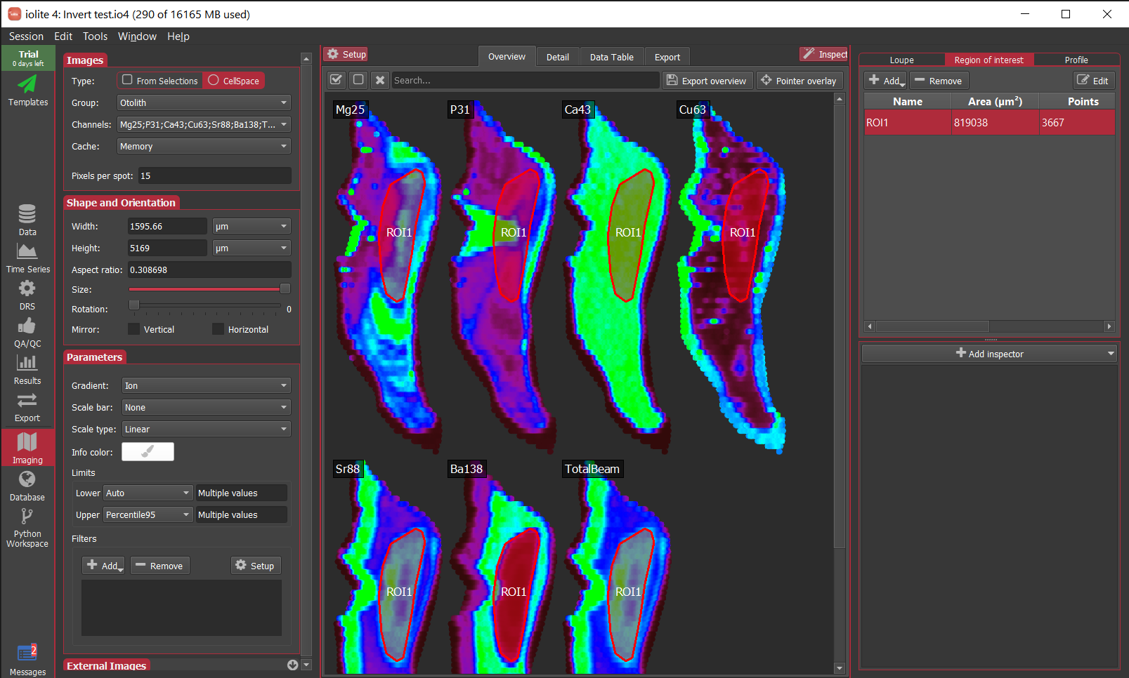
Then, you add a Clip image filter and select the ROI you want to use by name. The tools to add a filter are found in the Parameters section of the Setup panel on the left. When you click the Add button in the filters group you should select Clip. Initially, this may clip the entire image (i.e. it will disappear), but do not worry -- you can now select the name of the ROI to clip by using the Setup button near the filters list. To continue the example, from above I've selected ROI1 created above.
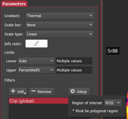
Finally, with those steps complete, the images will now only render in the areas covered by the ROI as shown below for the otolith example.
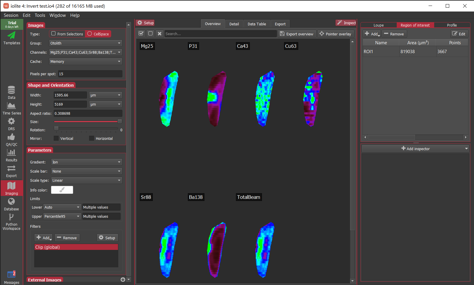
If you are bothered by a large amount of blank space when clipping to a significantly smaller area than was imaged, we've also just added the ability to turn a ROI into a selection group (right click on the ROI and select To selection group). If you're doing cell space imaging, this will have a similar effect as shown below for the otolith. Note in this case that the ROI now occupies the entire area resulting in less blank space.
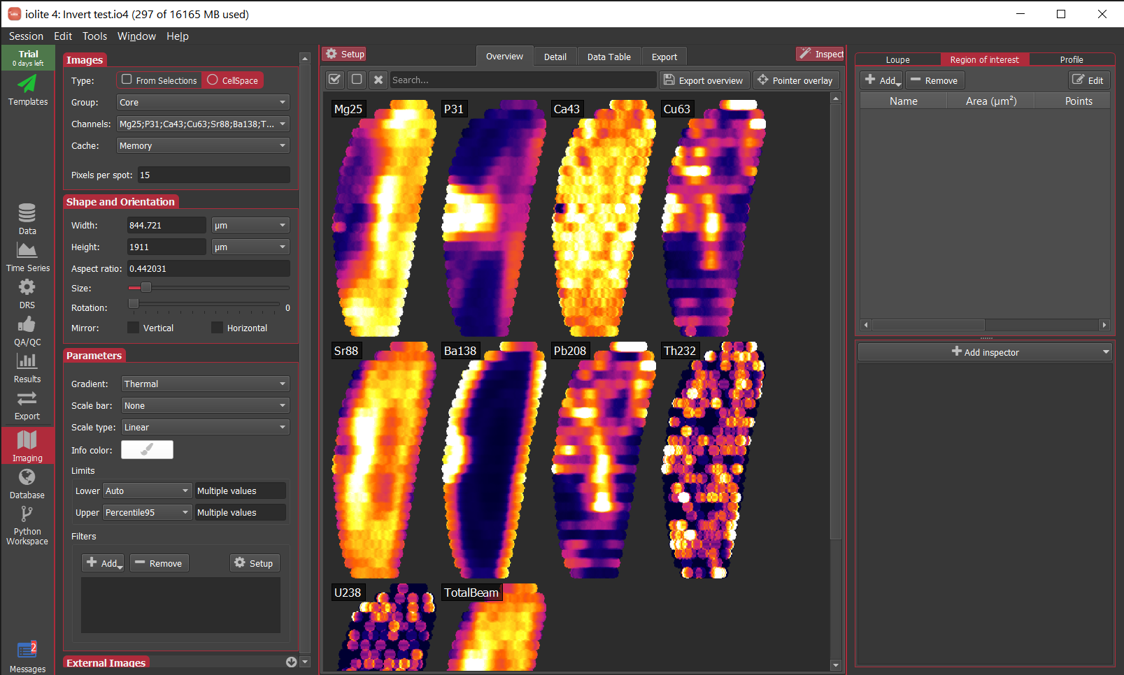
If you have any questions, comments or suggestions about this Note, you can discuss it here.
Using iolite 3/Igor Pro's color tables in iolite 4
Missing the color tables of iolite 3/Igor Pro in iolite 4? Read on to find out how you can transfer those color tables from Igor Pro to iolite 4!
Getting the color table data
Start Igor Pro, open the Command Window (Control+J for Windows, Command+J for Mac) and enter the following commands, followed by enter:
ColorTab2Wave ColdWarm; edit M_colors
This will open up a table of the red, green and blue values for the specified color table, in this case 'ColdWarm'. Note that the values are between 0 and 65535, which will be important later.
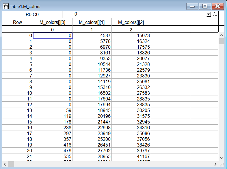
We can save this data out to a text file by going to Igor Pro's Data->Save waves->Save delimited text menu item. In the prompt, be sure to uncheck the option to write the wave name as shown below:
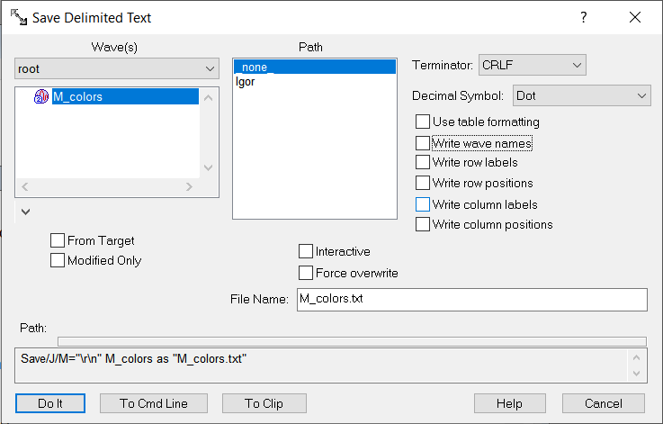
Adding it to iolite 4
Now we have the color table data in a format that we can easily read from python in iolite 4. Custom iolite 4 color tables are stored in the settings as a dict of lists, e.g.
color_tables = {
    'ColorTableName': [QColor(1, 2, 3), QColor(4, 5, 6), QColor(7, 8, 9)]
}
Where the parameters for QColor are the red, green, and blue values, but between 0 and 255 rather than 0 and 65535.
Knowing this information, the simple script below can be used to:
Get the existing (custom) color tables from iolite
Ask the user to pick a file
Read the file using pandas
Create a new list of QColors from the file contents while rescaling the values
Ask the user to name the new color table
Write the color tables back to iolite's settings
from iolite.QtGui import QFileDialog, QInputDialog, QColor, QLineEdit
from iolite.QtCore import QSettings, QFileInfo
import pandas as pd

# 1
settings = QSettings()
gp = settings.value('Imaging/CustomGradientPresets')
if not gp:
    gp = {}

# 2
fn = QFileDialog.getOpenFileName()

if not fn:
    raise Exception('No file')

# 3
df = pd.read_csv(fn, names=['R', 'G', 'B'], delimiter=' ')
d = []

f = 255./65535.

# 4
for i, r in df.iterrows():
    d.append(QColor(r['R']*f, r['G']*f, r['B']*f))

# 5
name = QInputDialog.getText(None, 'Preset name', 'Preset name', QLineEdit.Normal, QFileInfo(fn).baseName())

if not name:
    raise Exception('No name')

# 6
gp[name] = d
settings.setValue('Imaging/CustomGradientPresets', gp)
In action
After restarting iolite, you will now find your new color map as an option when choosing color scales in imaging. Shown below is our go-to otolith example in Igor Pro's cold warm.
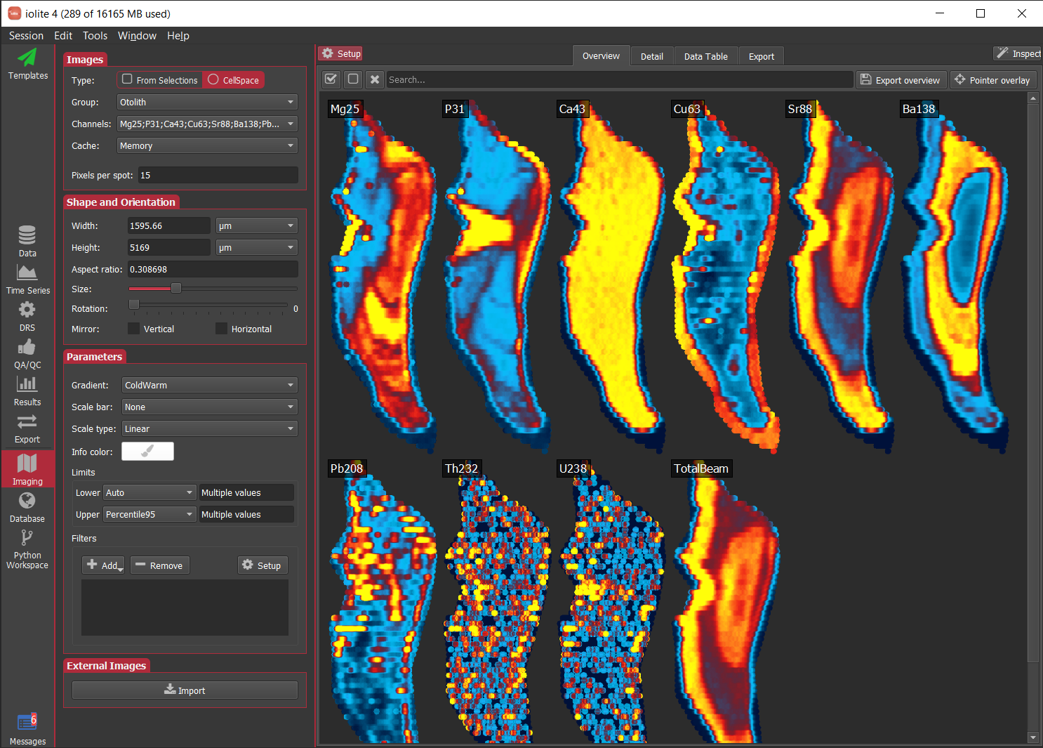
If you have any questions, comments or suggestions about this Note, you can discuss it here.
Using iolite's new Selection Checker tool
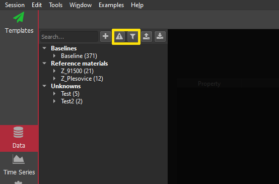
In the Selection Browser, there are two new buttons. One has an exclamation mark in a triangle, and you can click this button to run a check on your selections. If there are any issues with your selections, the color of the button will change: to orange if there are just warnings; or, to red if there are errors. There are also little error icons added beside any selection that has an issue in the list of selections. Again, if the icon is red, it is an error, and yellow if it is just a warning.
Also, now if you right-click on a selection in the list, an option to go to that selection in the Time Series View will appear. This can make it easier to find an selection with some sort of issue, and go straight to it to better understand what is going wrong.
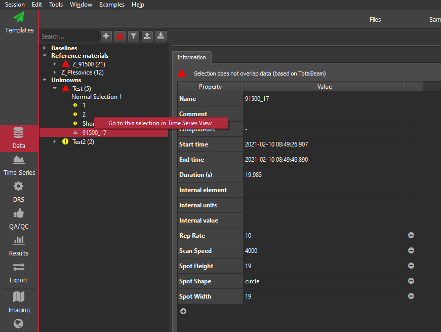
What are the errors and warnings iolite is telling me about?
At the moment, there is just one situation that will be reported as an "Error": where a selection does not overlap any measured data.
This can happen for a variety of reasons. For example, I was recently sent a dataset where an experiment was set up so that each spot ablation was treated as a separate sample by the mass spectrometer. This meant that each sample was in its own file. Normally, this is not a problem, however in this case for some reason the mass spec failed to measure a sample, so there wasn't a file for it and therefore no data were imported into iolite during this sample's ablation. But the laser log file still recorded the ablation, and so when the user created selections from the laser log file, there was a selection for the missing data. The missing data was for a reference material, and so the DRS the user was trying to run after creating the selections was reporting an error and wouldn't continue. The missing sample was one of hundreds in the session, and so it was very hard to find. With the new Selection Checker, this selection would now be highlighted as having an error. If you were to click on the selection in the Selection Browser, a message at the top of the window tells you why iolite thought it was an error. Deleting this selection allows the DRS to run to completion without any errors.
There are (currently) two sitations that iolite will flag as warnings (we may add others in the future): -1 Two selections within the same group that overlap in time; or -2 A selection contains very few datapoints (< 5)
The first is just a warning in case you've accidentally added the same selections twice (or more times). This can be very hard to distinguish visually if they have the same mean/2SE etc. It is just a warning because there may be valid reasons for overlapping selections. However, you should be aware that overlapping selections will mean that the same datapoints are included in more than one mean, reported as the average for the selection on export.
Similarly, very short selections may be valid because you're looking at a very small feature. However, typically you'll want more than 5 points to calculate a mean etc, which is why iolite will flag it as a warning so that you can review it. Also very short selections can be hard to see and delete when looking for errant selections.
Automatically checking for errors
iolite will now automatically check for selection errors when you click Crunch on a DRS, or when a DRS runs as part of a processing template. If there are any errors, the DRS/template will stop and tell you there is an issue so that you can fix it before continuing. Selection warnings will not stop the DRS/template from running, and it will continue but still report the warnings to the Messages View.
If you would like to turn this behaviour off, you can click on the wrench icon in the DRS View, and uncheck the "Check selections before crunching" option. iolite will not perform any check for errors or warnings when you click Crunch, and the DRS will not stop in the case of errors.
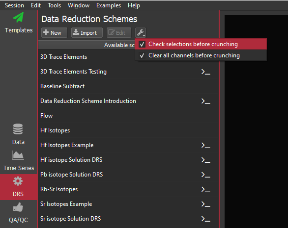
If you have any questions or suggestions for this feature, you can join the discussion here.
Importing Nu Plasma .run files into iolite v4
A quick look at the .run file format
Firstly, lets take a look inside a Nu Plasma .run file. If you open a .run file in a simple text editor (not Word) such as Notepad++ or Atom (both free), you can see that the first line contains the version information about the file. This is then followed by a bunch of lines with either a few numbers or some short text on it. This is the header information (usually just referred to as the "headers"), and we can mostly ignore it here. It does have information about which collectors were enabled etc, but there's not enough info here to import our data into iolite.
If you scan down, you'll see a line that just has the words "Spare Text" on it, usually around Line 46. This line marks the start of the actual data collected by the mass spec (and the end of the headers). Just above this Spare Text line is some information about the run, including the run start time, and the sample name entered when it was run. It also has which .nrf file was used to collect the data. A .nrf file is just an instructions file that tells the mass spec what masses to measure, how long to measure zeroes etc. In previous versions of iolite, we would decode that .nrf file to get the channel names. However, if your mass spec has a non-standard collector array (which is semi-common) we can't determine which masses were measured from the .nrf file, and everything breaks down... which is why we're editing some code here. Take note of the name of the .nrf file recorded in your file. We'll use that infomation later.

Below the Spare Text line are lines of comma-separated data. If you were to open this file in something like Excel, each value between the commas would be put into its own column. The number of columns depends on your setup, but the last three columns are usually a simple number that increases by 1 on each line; a quoted number; and a 0 or a 1. The first of these last three columns is just the measurement number (which is why it's incremented by 1 on each line). The second of these (the quoted number) is the timestamp for this measurement. If, for example, your mass spec is recording a measurement every 0.2 seconds the values in this column will increase by 0.2 on each line (there may be a second or so setup time). The final column represents whether this measurement was considered a zero or sample measurement, but we can ignore this because we'll create adjustable selections in iolite to determine what was zeros and sample after import.
Now to the actual data: each column represents a collector, and will become a channel in iolite. The channels start with the highest mass on the left. The mass difference between each column depends (again) on your setup. Naming these columns is what we'll be editing in our importer.
Creating your own importer
An importer in iolite v4 is just a python script. You can have as many of these as you like, and you just need to tell iolite where you're storing them so that iolite will use them when you try to import a file. You can set where your importers are stored in iolite's Preferences, in the Paths section, labelled Importers. By default, importers are stored in your iolite folder, which is normally in your Documents folder unless you chose a different location when you installed iolite. If you click on the -> button at the end of the Importers Path, it'll take you to the folder where your importers are stored. This folder might be empty: that's OK. You're about to put a script in this folder.
I would recommend that you download either Notepad++ or Atom so that you can edit your script. You can't do this in something like Word. Once you have your text editor installed, you can get the code. I've already written a basic importer script for .run files that does almost everything. You can just download this script and edit it to accept your .run files. You can download the file from here. Make sure that you click on the Raw button to see the raw code (rather than the webpage). Once you've got the raw code, copy all of it and paste it into a new blank document in your text editor. Then save it as something like "Sr_run_importer.py". Make sure that the file extension is ".py" so that iolite will know that this is a python script. Now we can edit it to make it work for your files.
Editing the importer
There are just three areas that you need to adjust for your file. The first is the metadata at the top of the script. When iolite reads the script, it needs to know what type of function this script performs (e.g. import data, DRS, QAQC module, etc). You just need to change the Name, Authors, and Description; the rest can remain the same. The Name is the only important one of these three, and should short but descriptive.
The next part to edit is the correct_format() function. When you select a file to import into iolite, iolite runs this function in each importer to see if the importer can load the file. The function searches the content of a file to see if it has something that identifies it as a file this particular importer can open and returns True (i.e. it can load this file) if it finds the text. In this case, we'll search for the .nrf line just above the Spare Text line described above. This line will be in every file and won't change (unlike the other metadata etc).
In this case, the .nrf file in our example was "Sr laser.nrf". We put this into the line starting with nrf_regex(the line underlined in yellow below; don't worry if you editor doesn't show the vertical lines like mine, these are just visual guides). We put a backslash before the '.' but otherwise it matches what was in our file's headers, and only includes the file name, not the full file path. Make sure that you get the uppercase and lowercase letters correct (the search is case sensitive.)
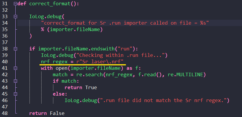
For extra points you can edit the debug message (Line 34 in our example) to say which importer was checking the file. This line is just there to help track whether the importer ran, so it's not essential to change this, but it can help track down issues later. There are two other debug lines on Lines 46 and 55 that you can also change if you like.
And now for the important part: to name the channels in your file. On Lines 111 and 112, you'll see two lists: a names_list and a masses_list. Each one is just a comma-separated list of names or numbers. The names_list is what each channel in your file should be called. You just need to update this list with your masses making sure that each channel's name is enclosed in single quotation marks, and is followed by a comma. This list also has the point number, measurement time and zeros column that I described above. Make sure you leave these in. Then edit the masses_list: it is in the same order as the names_list, but you don't need to include the point number, measurement time or zeroes column in this list. Make sure that each value is enclosed by single quotation marks.

Save your file and that's it: you're done. You can now try it out in iolite.
Using the importer
For iolite to recognise the new importer, you'll need to restart iolite. Once iolite has re-started, you should be able to see your new importer in the Plugin Manager. If you go to Tools -> Plugins -> Manage, iolite will show you a list of plugins that have been loaded in a list of the left hand side of the window. There is a search bar at the top of this list. Start typing the Name of your importer into this list, and it should appear and have a green light next to it if it was loaded properly. If it doesn't appear, make sure that the file you've been working on is in the folder listed in Preferences -> Paths -> Importers.
If your importer appears and is green-lit, you can try it out by clicking the Import file button as you normally would to import files into iolite. Select your .run file and it should import.
If it doesn't import correctly, you can check your debug messages in the Message View and contact us in the iolite forum for more help. If you have any other questions about loading .run files, please feel free to post here.
Selection refinement
Laser logs and mass spec sample metadata speed up the process of creating selections in iolite considerably. However, sometimes we want to further refine those selections for a variety of reasons. For example, maybe the laser log and mass spec don't quite agree on the timing of things, or you want to automatically avoid parts of the signal where you've ablated through the target. Read on to find out more about iolite's new selection refiner tool!
Overview of the user interface
The selection refinement tool (included in iolite 4.5.2+, some features described in soon to be release v 4.5.3) can be accessed via the Tools → Refine selections menu item. A dialog similar to below will appear:
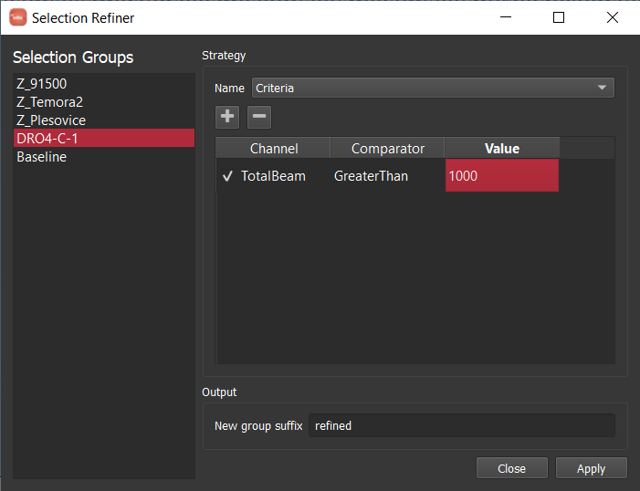
In this dialog there are a few different areas of note:
The Selection Groups area on the left. In this list, you select the group(s) that you would like to apply the refinement strategy to.
The Strategy area comprising the bulk of the window. In this area, you select the strategy type at the top and the settings for that strategy are shown below.
The Output area at the bottom. In this area, you specify the suffix that will be used when refining the selections in a group. For example, if you have selected a group called 'Unknowns' and the suffix is ' refined', a new group will be created called 'Unknowns refined' that contains the selections of 'Unknowns' that have been modified by the selected strategy.
Refinement strategies
There are a number of refinement strategies included with this tool and you can also add your own since this plugin is python-based. The included strategies are briefly described below.
Criteria
This strategy is similar to 'automatic selections from channels'. It finds the longest segment of each selection that matches a list of criteria. For example, you could use this strategy to adjust a selection to avoid inclusions or parts of a zircon analysis with high 204Pb.
Mean shift clustering
This strategy uses mean shift clustering on the data for the specified channels during each selection to find the cluster in the selection. For example, you could use this strategy to adjust a selection to the dominant phase of an analysis.
Rolling standard deviation and error
This strategy searches the selection for the segment with the lowest standard deviation or standard error for the selected channel. For example, you could use this strategy to find part of a selection that has the most homogeneous 207Pb/206Pb as shown below where the full selection (red ellipse) was refined based on 207/206 (blue ellipse).
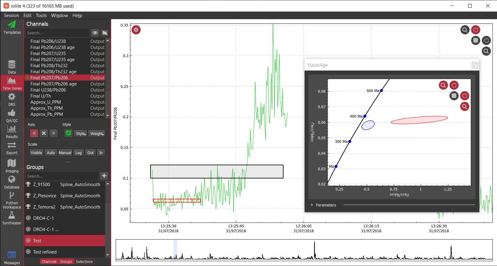
Extremes
This strategy looks for the segment (with a minimum length criteria) that minimizes or maximizes the selected channel on average. For example, you could use this strategy to adjust a selection to match the highest (perhaps to avoid drill through) or lowest (perhaps to minimize discordance) segment. Shown below is the same example as above but instead refining the selection to minimize discordance (resulting in a very similar sub-segment).
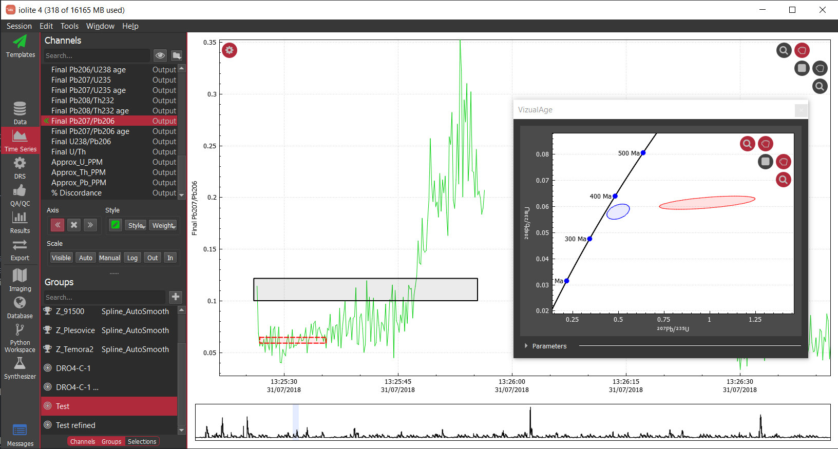
Synchronize
This strategy adjusts the selection such that it is optimally synchronized with the data within some search window specified as the maximum time difference. For example, you might use this to correct small differences in timing between the recorded mass spec data and the laser log.
The end
That was a quick look at the new selection refinement tool in iolite 4. If you have any questions, comments or suggestions about this Note, you can discuss it here.
Filling in the blanks (in imaging)
Sometimes when imaging we purposely leave space between spots to save time or maybe there is a gap in your image from an instrument glitch. In either case, the cell space image will contain regions of null data, and often we would like to replace those missing parts to make a better looking image. Read on to find out more about how you can do just that with iolite's (v4.5.2+) new Replace Null imaging filter.
How it works
Consider the following matrix of dots (not to be confused with an image!) where the red dots represent good data and the black circle represents a missing or null bit of data in the image's matrix.

There are, of course, a number of ways we might calculate the values for our missing dot. The simple approach taken by this filter is to consider a shape surrounding the missing data and use the non-null data in that region to compute the value, but how large should the region be? What shape should it be? How should the value be calculated? How do we handle edge cases? All of these things can be controlled by the user in the filter's settings widget shown below.
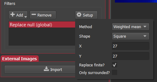
Method This controls whether the value will be computed as a mean, median, or weighted mean.
Shape This controls the shape of the region around the null data to be used in the calculation, currently one of: circle, square, or diamond.
X, Y These parameters control the size of the region in pixels (so be mindful of your pixels per spot size). In the dot images above, the region would have X = 3 and Y = 5.
Replace finite? This controls whether finite data will also be replace, effectively smoothing the entire thing.
Only surrounded? This controls whether to replace null data only when it is surrounded by good data. To be considered as surrounded the region must not have any completely null halves. In the right dot image above, the right half of the region is completely null, and therefore this data point would not be replaced.
Now let's consider some examples!
Missing line
The first example we will consider is that of a missing line of data. Shown below is a series of images with no filter on the left, and the null replacement filter with "only surrounded" off and on in the middle and right, respectively.
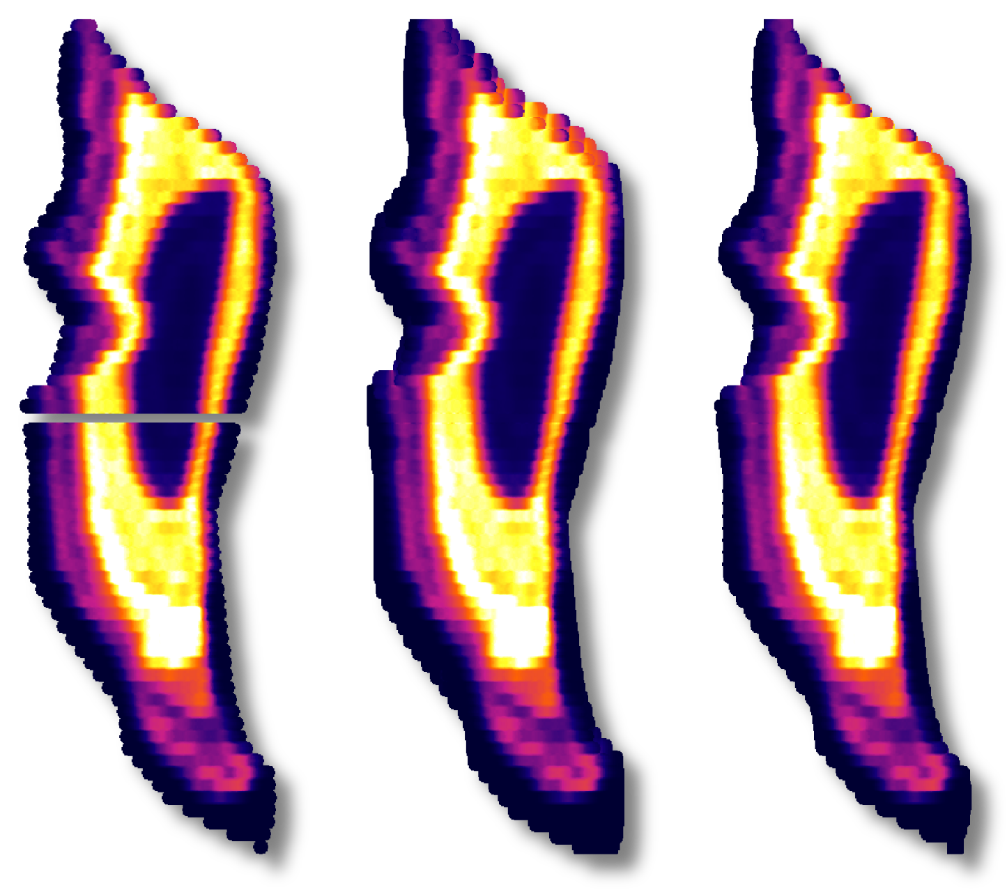
This sequence demonstrates how by replacing null data that is not surrounded we grow our image by filling in the data around the perimeter. By limiting our filter to only replace surrounded data we achieve the desired effect. For this example, I wanted to use the data above and below the missing line so I used X=1 and Y slightly greater than the pixels per spot.
Grid of spots
Next we will look at an example where a series of spots were patterned over an area. If we were to image this dataset in cell space without filtering, it looks as shown below on the left.

In this case, I played around with the settings quite a bit and ended up using a region a bit more than 2x the pixels per spot with a weighted mean.
And that's it!
Click here to discuss.