Database

Overview

iolite's Database tool will create an SQLite database from your existing iolite session (.io4) files. It does this by reading through your session files and extracting the results for each selection. For example, if you were to import a typical session, there would be a result for each input, intermediate and output channel for every selection (including baseline selections).

The advantage of a database is that you can import all your sessions to determine parameters such as inter-session reproducibility, long-term trends in your data, and many other things that might not be apparent when you look at sessions individually. You can also collate multiple sessions to be able to view all results in one place, e.g. all sessions for an overarching project. We have also built in tools to sort, filter and even plot your database results. For even more flexibility and power, you can interact with the database via iolite's python interface so that you can run python scripts to create plots, calculate new results, and store or retrieve data from other data repositories.

The database file created is a standard SQLite database (.db) file. This means that your database can be opened with other third-party programs (e.g. the free and open-source DB Browser for SQLite).

Tip

You can also import iolite v3 .pxp files, as well as Excel spreadsheets. Just remember that if you're storing date/times in your Excel spreadsheet, it should be in the following format: "yyyy-MM-dd hh:mm:ss.zzz". If you're worried about how a file might import, you can create a blank database and import your file to see how it goes.

Associating external results

As noted above, your database will contain a row for each selection and a column for each result/channel in your experiment. However, it is likely you'll also want to link external data with your results. For example, you may want to associate external data such as IGSN, batch labels, sample type, etc with a particular result. You can do this by adding 'properties' to selections. Selections already have a variety of default properties, such as start and end time, duration, spot size etc (see Fig. 21). However, you can add additional properties to selections to link the results associated with that selection with other information. You can, for example, add the IGSN for the sample by adding a property to the selection, renaming the property to 'IGSN', and setting the value to your IGSN.

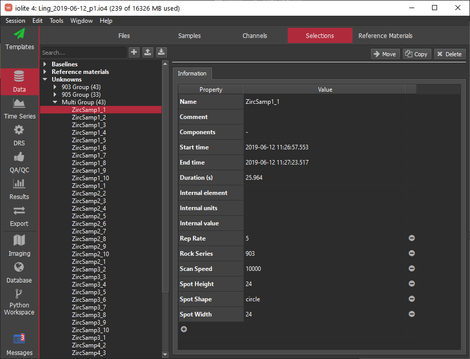
Fig. 21 iolite's Selection Browser, showing properties for a single selection "ZircSamp1_1". Note the '+' Add Property button at the bottom of the properties list, beneath 'Spot Width'. This button can be used to add properties to selections.

Of course, manually adding a property to hundreds of selections would be time consuming and inefficient, so we've come up with some ways to add properties to multiple selections more efficiently. The first method is to add a property to all selections within a group. This can be quite powerful if your selections are already grouped according to some shared property (e.g. sample group, mount, etc). You can add a property to every selection within a group by clicking on the group's name in the Selection Browser. This will show you the group's properties, such as the group's name and the number of selections within the group. If you add a new property here, it will add that property to all selections with the group. If you set the value here, all selections within the group will have that value.

While this is a quick and easy way to apply a single value to all selections within a group, you may want to apply various values to each selection. You can do this via a couple of simple python scripts. The first will export all the selection names to an Excel spreadsheet. You can then add columns to this spreadsheet and import the spreadsheet using a second python script. This second script will add a property for each column in the spreadsheet. For example, if you have a column called 'Batch No', all selections that are listed in the spreadsheet will be given a new property called 'Batch No'. The script looks through every selection within the group to match up it's name with an entry in the spreadsheet.

Below is a guided example on how to do create a database from a single session file, including how to add properties to individual selections manually and using the python scripts described above. Finally, we'll create a quick plot of our results, and export a subset of results to an Excel spreadsheet.

Quick Example

For this example, we'll be using an example U-Pb dataset. Please note that you can create and interact with your database with any type of experiment, not just U-Pb data.

Here is a link to the U-Pb example dataset: click here.

There are two files in the example dataset: a U-Pb session file (U_Pb_Example_DB.io4) and a spreadsheet of dummy IGSN, field trip codes, and publication codes (sel_labels_example_filled.xlsx).

In the example below we'll create properties for our selections in two ways: manually; and, using the python API. Remember that the properties will become columns in our database that we can then use to filter and/or sort our data by.

Manually adding properties

1. Open the session file (U_Pb_Example_DB.io4).

2. Go to the Selection Browser in the Data View. Click on any selection in the DRO group. Double-click in the Comment field, and write a comment such as "This selection has a comment". We'll be able to find this comment later in our database.

3. Now lets add a property to a selection manually. Click on the + button at the bottom of the properties of any selection in the DRO group to add a new property. Rename the new property to something like 'Rock series' (or anything really).

Tip

Property Names without spaces can be easier to handle when writing arithmetic. If you think you'll be using your property in calculating other results, perhaps avoid spaces or special characters such as '\\'

Click on the value for your new property and type in anything (e.g. 'GSV2020_153').

Adding properties using the python API

4. You can add individual values to each selection in a group using the python API. First, to export our selection names to an Excel spreadsheet, you can copy the following code to the Python Workspace in iolite and click Run.

from iolite.QtGui import QFileDialog, QWidget, QInputDialog
from iolite.QtCore import QSettings

import pandas as pd

grp_list = data.selectionGroupNames(data.Sample)

grp_name = QInputDialog.getItem(QWidget(), "Select a group:", "Group", grp_list, False)

grp = data.selectionGroup(grp_name)

df = pd.DataFrame()

selNames = []

for sel in grp.selections():
        selNames.append(sel.name)

df['selection label'] = selNames

file_name = QFileDialog.getSaveFileName(QWidget(), 'Select save location', 'sel_labels.xlsx')
if len(file_name) > 0:
        if not file_name.endswith('.xlsx'):
                file_name += '.xlsx'

        df.to_excel(file_name, index=False)

This will create an Excel spreadsheet with the selection labels in the first column. You can then add columns to this spreadsheet and import the values into iolite. I have created an example spreadsheet (sel_labels_example_filled.xlsx) where I've created some dummy IGSN, fake field trip numbers, and some fake references to cite.

5. You can import these values to automatically add the property and property values to our selections using the following script. When you run it, it will ask you which spreadsheet file to import. Select the example spreadsheet (sel_labels_example_filled.xlsx). It will then ask you which group to match with the sample labels (in case you had two groups with the same label). You can copy and paste the following code into a tab in the iolite Python Workspace.

from iolite.QtGui import QFileDialog, QWidget, QInputDialog
from iolite.QtCore import QSettings

import pandas as pd
import math

file_name = QFileDialog.getOpenFileName(QWidget(), "Open Sel Properties Excel File", "", "Excel Files (*.xlsx)")

df = pd.read_excel(file_name)

grp_name = QInputDialog.getItem(QWidget(), "Select a group:", "Group", data.selectionGroupNames(data.Sample), False, False)

grp = data.selectionGroup(grp_name)

for index, row in df.iterrows():
        import_label = row['selection label']
        for sel in grp.selections():
                if sel.name == import_label:
                        for col in df.columns:
                                if col == 'selection label':
                                        continue

                                sel.setProperty(col, row[col])

Once you have run this script and imported your dummy values, you can see them in the Selection Browser. Click on a few different selections to see that the properties do not have all the same values.

6. Now save your session. This will store the selection properties we've just created in the .io4 session file.

Creating a new database

7. Now we'll create our database. Go to the Database button on the left hand side of the iolite Window. Here's a quick overview of the interface:

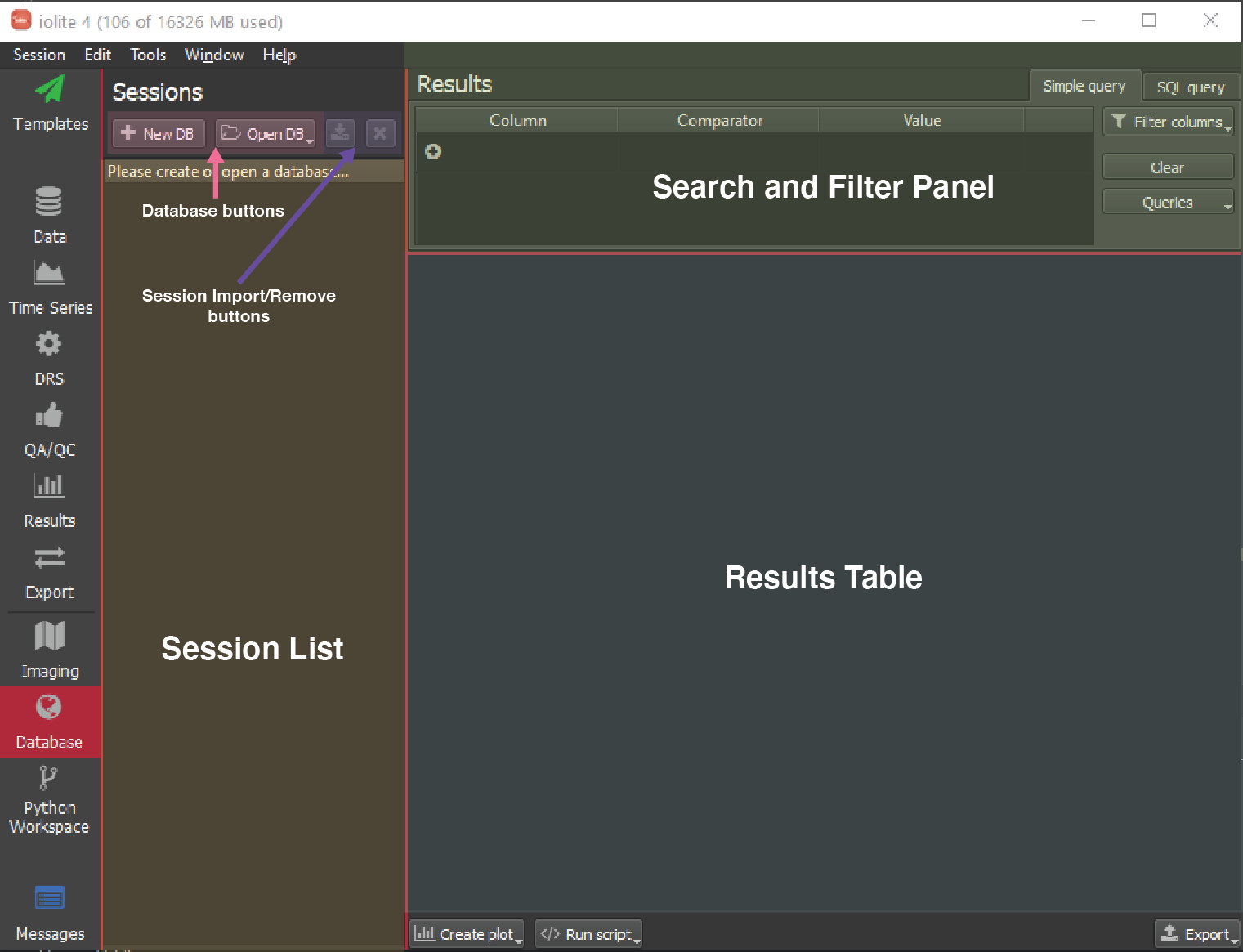
Fig. 22 Schematic of iolite's Database tool user interface

Click the + New DB button. Choose somewhere on your computer where you have full read/write access (e.g. your Documents folder). Call your database something obvious, such as "TestDatabase.db".

8. We now have an empty database. Let's import some sessions. Click on the Add Session button and select our session file we saved in Step 5. You should now be able to see your file in the list of imported sessions, along with the number of selections in the file, and the date of the session. You'll also be able to see all the selections in your file in the Results Table. If you scroll the table across, you'll see that there are a series of metadata columns (e.g. Spot Shape), and then a column for every channel including input, intermediate and output channels, and our custom properties that we added ('IGSN', 'Field Trip' and 'Publication')

9. We can do some simple filtering of our results using the Simple Query search and filter panel. Let's show only reference material results (which in this case will include 91500, Temora 2 and Plesoviche). Click on the + button in the search and filter panel, just beneath where is says Column. This will add a new filter. Double-click where is says "Name" to set the column to filter on, and change it to Group Type. We can keep the Comparator the same, but double click on this to see what options are available. Double-click in the Value field and type "Reference Material" exactly (it is case-sensitive). When you hit Enter, you'll see that the table now only shows your reference material results. You can save your queries using the Queries button on the right of the search and filter panel.

10. You can filter which columns are shown in the Results Table using the Filter Columns button in the top right. Columns are added to the table in the order that they are selected. Columns are arranged by their type (metadata, input, intermediate, output, etc). Columns that were created by a DRS (e.g. intermediate and output channels) are listed according to the name of the DRS that created them. You can select all channels in a section by clicking the All button at the bottom of the section. To deselect all channels in a section, click the None button. To remove all filtering, click None for all sections.

10. We can create a plot of these reference material results using the Create Plot button towards the bottom left. Click the button and a new empty plot will appear as a new window. We'll just do a quick plot of 206Pb/238U ages for our reference materials. Click the Add Graph button in the top left of this window to add a new trace to the plot. In the window that appears, for the Y values, select Output -> Final 206Pb/238U age. For the X values, just click Count at the bottom of the list. Then click OK. Our data is on the plot, but we can't see it because it's too zoomed in. Right-click on the plot and select Rescale to zoom out to show all data. You can see that we have a line graph of our data. Let's change it to circle markers and add some tools to our graph. Click on the Settings button in the top right of our plot window. In the Tools section, select all of the X and Y pan and zoom tools. Then in the Items tab, click on the Main item in the list. This is where the individual 'graphs' are listed. Here 'graph' means the plotting of one variable against another. You can plot as many variables as you like and they'll appear in this list, under 'main'. We just have one graph called Graph 1. To change it from a line graph to markers, uncheck the Line option, and check the Marker option. Then, in the symbol dropdown menu, select 'disc'. You can now close this Settings window. You'll then be able to see that we have our reference material results plotted as discs, and we now have our pan and zoom tools in the top right of our plot. You can click these tool icons to turn them on/off to move around and zoom in/out on your data. We can close our plot for now.

11. You can export a subset of your data to an Excel spreadsheet. We can export our reference material results in this example by clicking the Export button (bottom right) and selecting Excel. This will export all the values currently in the table (i.e. only the results that match the current filtering criteria). If you want to save all of your data as a separate file, clear all filters using the Clear button in the Sort and Filter Panel.

12. Just as a quick demonstration of more advanced features, let's have a look at the SQL Query tab (top right of main window). Click this tab to show the SQL search panel. Here you can write more advance SQL queries. If you're not interested in SQL, feel free to skip to the next step. Firstly, lets start with an example where we select Reference Materials and Samples (i.e. not baselines), and specify how our results are ordered. Type the following into the SQL query panel and press the F5 button (Cmd+r on Mac) to run the query:

SELECT * FROM results WHERE `Group Type` = 'Reference Material' OR `Group Type` = 'Sample' ORDER BY `Group Name`,`StartTime`

Your Results Table will now only show reference materials and samples, ordered according to group name and then by start time. Using this interface, we can also see other parts of the database. For example, if you type the following and press F5 (or Cmd+r on Mac):

SELECT * FROM sessions

you can see that we are now viewing the sessions table. Here you can see that the DRS and Spline settings have been recorded as JSON. This table is a bit boring in this example because we have only one session imported into our database, but as you import more sessions, this table will contain more information.

Tip

You can copy the DRS and Spline settings data (as well as any other data in this table) using Ctrl+c (Cmd+c on Mac). You can then paste the data into another program (e.g. NotePad etc). Pasting data into this table has no effect.

If you type the following and press F5 (Cmd+r on Mac):

SELECT * FROM channels

you can see the third and final table in the database: the channels table. Here you can see information about each channel, such as which sessions include the channel, and for output and intermediate channels, which DRS created the channel.

Creating new columns: A simple calculation

13. Now we'll run a simple python script that acts on our database results. You can copy and paste the following code into a simple text editor such as Notepad ++, or Atom. Save the file as a .py file (e.g. discord.py) somewhere you'll find it again. Then click on the Run Script button (bottom left). Find the script you just saved and click Open. The script will run, and a new column will be added to your database called 'My discordance' (you may have to scroll all the way to the right to be able to see this new column).

import numpy as np

# Get some data from the database to use in calculation
t76 = np.array(db.column('Final Pb207/Pb206 age'), dtype=np.float64)
t68 = np.array(db.column('Final Pb206/U238 age'), dtype=np.float64)

# Do the calculation
disc = 100*(1 - t68/t76)

# Add the column to the database
db.appendColumn("My discordance", disc)

print("Finished adding discordance")

From version 4.4.0, iolite comes with more example python scripts showing some of the things possible with iolite's Database feature. These examples should give you a feel for some of the things that are possible, but certainly not all. The scripts are located in your iolite folder, which will likely be somewhere like C:UsersmyUserNameDocumentsioliteScriptsDatabaseor similar on Mac. If you create your own python scripts that you think the community would benefit from, please feel free to share them on the iolite forum.