User Interface Guide¶

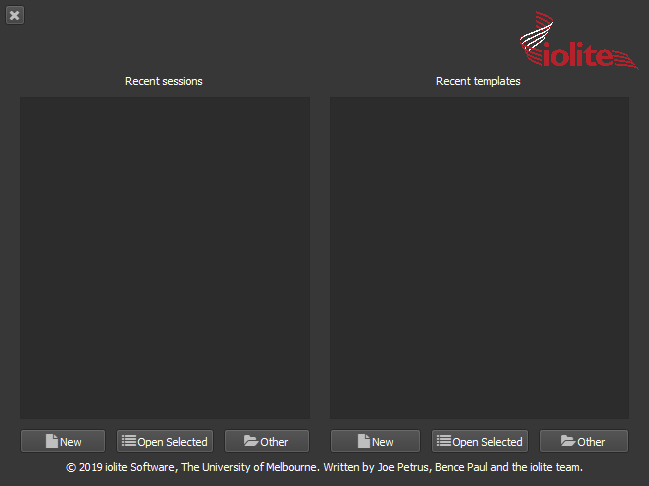
When iolite first starts, you should see the Welcome Window. This window shows recent Sessions on the left and recently used Processing Templates on the right.

Hint

A "session" is a self-contained experiment. Conceptually, it is typically from when you turn your mass spec on until you turn it off again. It's usually un-wise to include two experiments where the mass spec has been switched off and on again as one session. This is because the results from one session will affect the splines of the second, and if you have retuned your instrument, or if gas flows are different etc etc, then it's likely you don't want this interaction to happen. From a file perspective, iolite saves all your channel data, all your selections, your DRS settings and your calculated results in a HDF5 file so that you can reload it to work on it later. This is exactly analogous to .pxp files in previous versions of iolite.

You can load any listed session or template by double-clicking on it, or by selecting it and clicking Open Selected. If you have not saved any sessions or templates, both these lists will be empty to start with. You can load sessions or templates not listed by clicking the Other buttons.

To start a new session, click the New button on the far left. (The New button on the right opens a new session starting in the Templates view, described below).

The figure below shows the iolite v4 user interface:

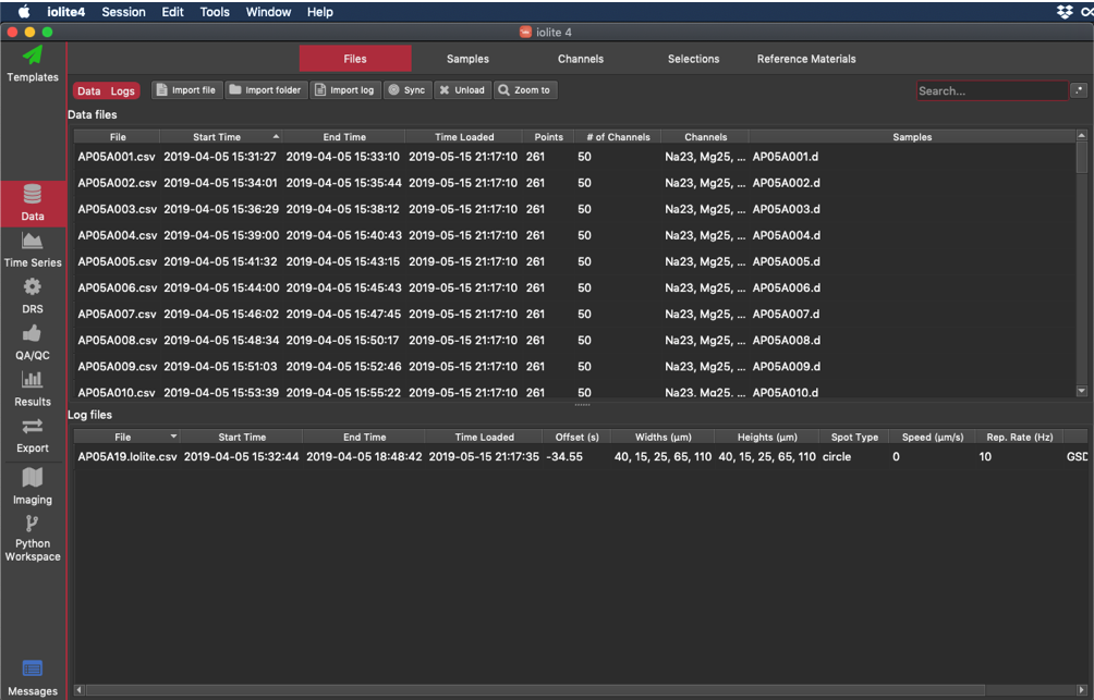
Although the Mac version is shown, it is the same on Windows, with the exception that there is no iolite4 menu. The items in this menu can be found in the Session menu.

Menu Bar¶

Along the top of the screen there is a menu bar with Session, Edit, Tools, Window and Help.

Session menu: here you can save and load sessions. See the hint above about Session files. You can also import iolite v3 .pxp files here. there are options for importing data here too, but we recommend that you use the Files Browser, described below under Files Browser, for loading your data. There is also the Preferences item, which is described in detail in the Preferences section of the Installation instructions.
Edit menu: contains undo and redo capabilities for certain actions (e.g. undoing deletion of selections).
Tools menu: This contains many useful tools, such as Automatic Selections from Channels, the iolite v3 Reference Material file converter, the Data Syncer for split stream experiments etc.
Windows menu: shortcuts for the tabs along the side of the main window (described below). Also has the Notes action. Use this to show the Notes dock, where you can record notes along with your session.
Help window: Useful help functions, including the Interactive Help feature. You can also activate the Interactive Help by pressing F1 at any time. Will show a help dock with help for whichever part of iolite you are currently using. Also includes the Check for Updates item where you can see if you have the latest version of iolite. If not, you will be prompted to download the latest version and it will automatically install the new version for you. Very handy! Requires an internet connection.

Hint

In the Help menu on Windows, there is an About iolite4 item (this is under iolite4 -> About iolite4 on Mac). Here you can see what version of iolite you're currently using. You can check for updates at any time using the Check For Updates item in the Help Menu (on both Mac and Windows). If an update is available, it will automatically download it, verify it, and install it. This feature requires an internet connection.

Main iolite Window¶

Along the left hand side of the Main Window, there are a series of tabs, starting with Templates at the top, and Messages at the bottom. We refer to these as Views as they are different ways to view the data in your current session. By default, you start in the Data Browser View. Each of the views are described below.

Data Browser View¶

This tab allows you to see all the data you've loaded, as well as information about your selections, channel data and reference materials. These pieces of information are arranged by tabs at the top of the window.

Files:

The Files Browser, showing what mass spec and laser log files have been loaded, and some information about what was in each file

Samples:

The Samples Browser, showing information about the samples that were recorded in the mass spec and laser log files you have loaded

Channels:

The Channels Browser, showing information about the channels you have loaded from mass spec files (input channels), and calculated channels (Intermediate and Output channels).

Selections:

The Selections Browser, showing information about any selections you have created

Reference Materials:

The Reference Materials Browser, showing which reference material files have been loaded.

Reference Materials Browser

Files Browser¶

Use the Files Browser to import mass spectrometry data and laser log files and view both mass spec and laser log files that have been imported. The main screen is divided into two parts: the top half is for mass spec files (Data files); the bottom half is for imported Laser Log files. After a file is loaded, it will appear in the list of files loaded.

How to import data¶

Hint

If you're loading an Agilent or X-Series II file, you should set your timestamp format before clicking the load button. Go to Session > Preferences (iolite 4 > Preferences on Mac) or press Ctrl + , (Cmd + , on Mac). Then on the Import tab choose the correct time stamp format. Your selection will be saved for all future imports. See also the Preferences section of the Installation instructions.

Click Import File or Import folder to bring up the file or folder browser window, respectively.

In the browser window, search for the file or folder you want to open. Once you have found it, double-click it or select it and then click Open.

You should check the Messages (blue icon at bottom of left side menu) after each import to check that the files imported correctly.

How to import laser log files¶

Click Import Log to prompt the file browser window.

Select the log file you want to use and then click Open. You must have already imported the associated mass spec data before importing the laser log.

In the sync window, you can:

Adjust the time overlap between the laser log and the mass spec data. To do this, drag the laser data (the green trace) by holding down the Shift key and clicking and dragging the trace.
Zoom the x axis using the mouse scroll button.
Change the x axis extent by clicking and dragging the graph.
Use the "Laser Offset" variable display at the bottom left to set an exact offset, if known for your system. The up/down arrows move in 1 s increments, but you can manually type in the offset for finer control.
Check the "Auto sync?" checkbox at the bottom to automatically sync your laser log file with your mass spec data.
Use the "Sync channel" popup to choose the channel you want to sync your laser log file with.
Use the "10ⁿ" button to switch between log and linear y scaling.
The "in range" field allows you to define the search window for the auto-sync feature. For example, if your mass spec data spans a time period of one hour, using a value of 2 for "in range" will look for an overlap with the laser data up to one hour before the start of the mass spec data and one hour after the mass spec data ends. This is useful if your datasets are initially quite far apart in time. Increase this value to help with auto-syncing your data, or manually adjust your data.

Once you're happy with the offset, click the Done button to finish the import.

If you want to re-sync a laser log file, select the log file in the list of imported laser log files, and click the Sync button.

From the Files Browser you can also:

Unload any file by selecting it in the list and clicking the Unload button.
Hide the logs or data part of the interface by clicking on the Data | Log button in the top left (both selected and red by default).
Adjust the syncing of a laser log file by selecting the file and clicking the Sync button. This will show the laser log sync window again so that you can adjust the sync.
Zoom to the extent of a file in the Time Series view by selecting it in the list, and then clicking the Zoom to button.

Tip

The 'Zoom to' option is best to use if you have imported multiple files and if you have a second iolite window open to the Time Series browser, so that you can view the zoom-to action simultaneously. To open a new iolite window go to Window > New iolite Window or press Ctrl + = (Cmd + = on Mac). Then select the Time Series browser and add a Channel to view. In the first window, select an imported file from the Data files list. Then click the Zoom to button and watch the Time Series view in the second window change.

Samples Browser¶

The Samples browser shows a list of samples that have been imported from both mass spec files and laser log files. Samples within mass spec data files are listed in the top half of the screen and samples within laser log files are listed in the lower half of the screen. Some mass spec file formats only contain a single sample (e.g. Agilent) and some contain many samples within the same file. You can hide or show the Data (mass spec samples) or Log (laser log samples) Files by clicking on the Data | Logs buttons at the top left, which are both selected by default. Laser log samples correspond to entries in the laser log file (e.g. each spot or scan-line).

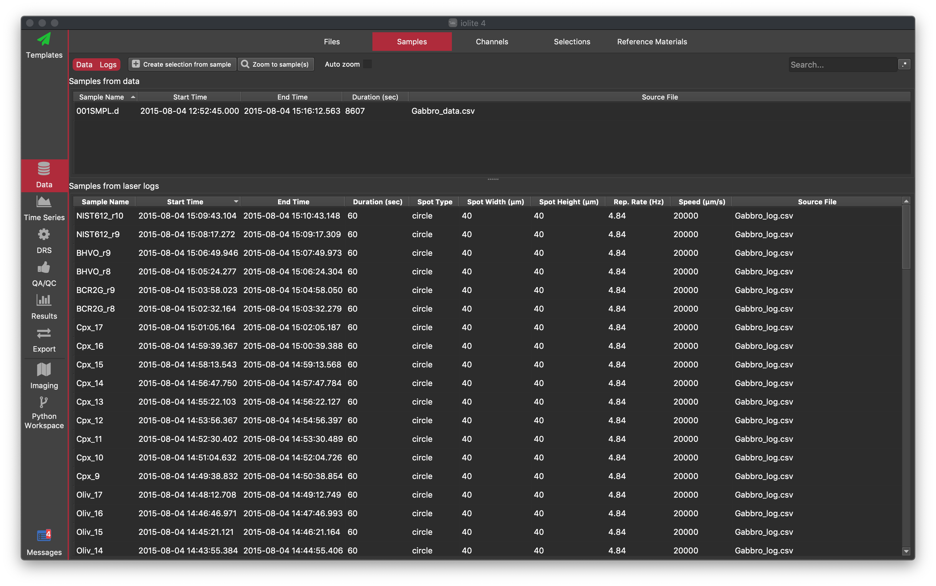
The following information is available for each mass spec sample: Sample name, Start time, End time, Duration and Source file.

Laser log samples have columns for start/end time, duration, spot type (circle/rectangular) Spot Width/Height, laser repetition rate (Rep. Rate), scan speed and source file.

You can sort the samples by any of these columns by clicking on the column label. This can be helpful when you have imported data from several files, or if you have different ablation durations within an experiment.

How to create selections from samples¶

In any of the samples list, select the samples from which you would like to create selections. You can use Ctrl + A (Cmd + a) to select all samples in the list. This is especially handy if you use the search feature (see hint below).

Hint

You can also search for selections using the Search... input field in the top right of the window. This search tool is case-sensitive. Advanced users can check the .* button to use Regular Expressions for selecting samples.

Click the Create selection from sample button.

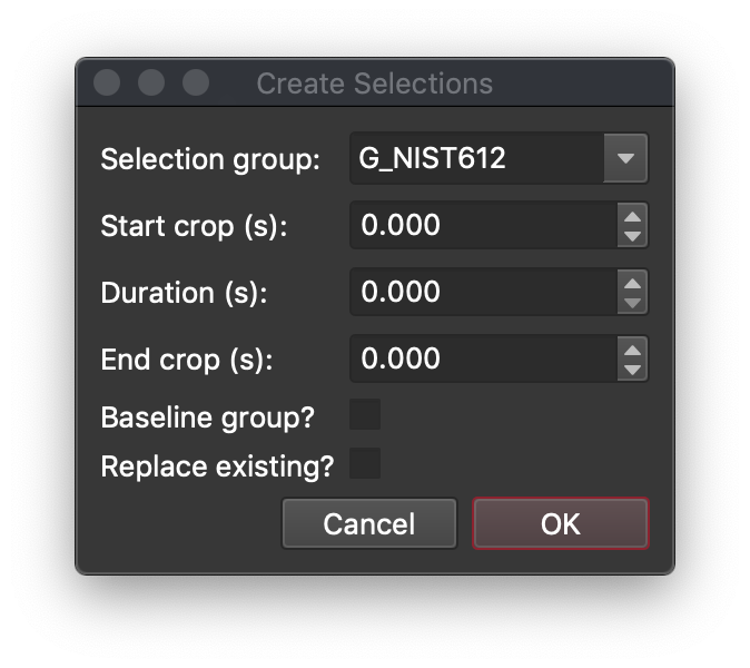
In the Create Selections window (above), iolite will try to automatically guess which selection group to add the selections to by the sample labels. If you want to use a name not in the list (e.g. for baselines), you can just start typing into the "Selection group" field. You can choose the start crop and the duration or the start crop and duration. If duration is any value other than 0, End Crop will be ignored.

Note

If you are creating baseline selections, you must check the "Baseline group" checkbox. This tells iolite which group contains the baselines.

If you would like to overwrite the existing selections in the selected group (if it already has selections in it), check the "Replace existing?" checkbox.

Click the OK button to create your selections.

Remember: You can check the messages logged during sample selection creation by going to the Messages browser. There you can find information on the number of selections added, the group to which these selections were added to, the start and end crop times used, and the total number of selections in a group after creating the selections. This information can be useful when trying to re-create selections.

Zoom to sample(s): You can zoom to a sample selected in the list by clicking the "Zoom to sample" button. This will zoom the Time Series View to the selected samples time extents. If you check the "Auto zoom" check box, the x axis of the Time Series View will zoom to the currently selected sample as you move through the list (e.g. by moving through the list with the up and down keys).

Channels Browser¶

The Channels browser allows you to access information about the channels within the session. The left-side window shows a list of all existing channels. Channels are arranged in the list according to:

Input (the raw data read from the mass spec file).
Intermediate (channels created during the execution of the DRS, but that are not considered part of the output).
Output (channels from which the final results are calculated from). For example, the final concentration channels, or final corrected ratios (depending on the DRS used).

You can select channels from any category by clicking on the expand arrow, and then clicking on the name of the channel you wish to select. You can also filter the channels in each category by typing into the Search... box at the top of the list.

The right-side window displays information about the selected channel. There are three information tabs:

Information: This tab shows general information about a channel, including the number of points, what machine it was imported from and the start and end time of data within the channel.

Hint

If using the Pettke Limits of Detection calculation, this is where you should set your dwell times (if not automatically loaded from your mass spec file).

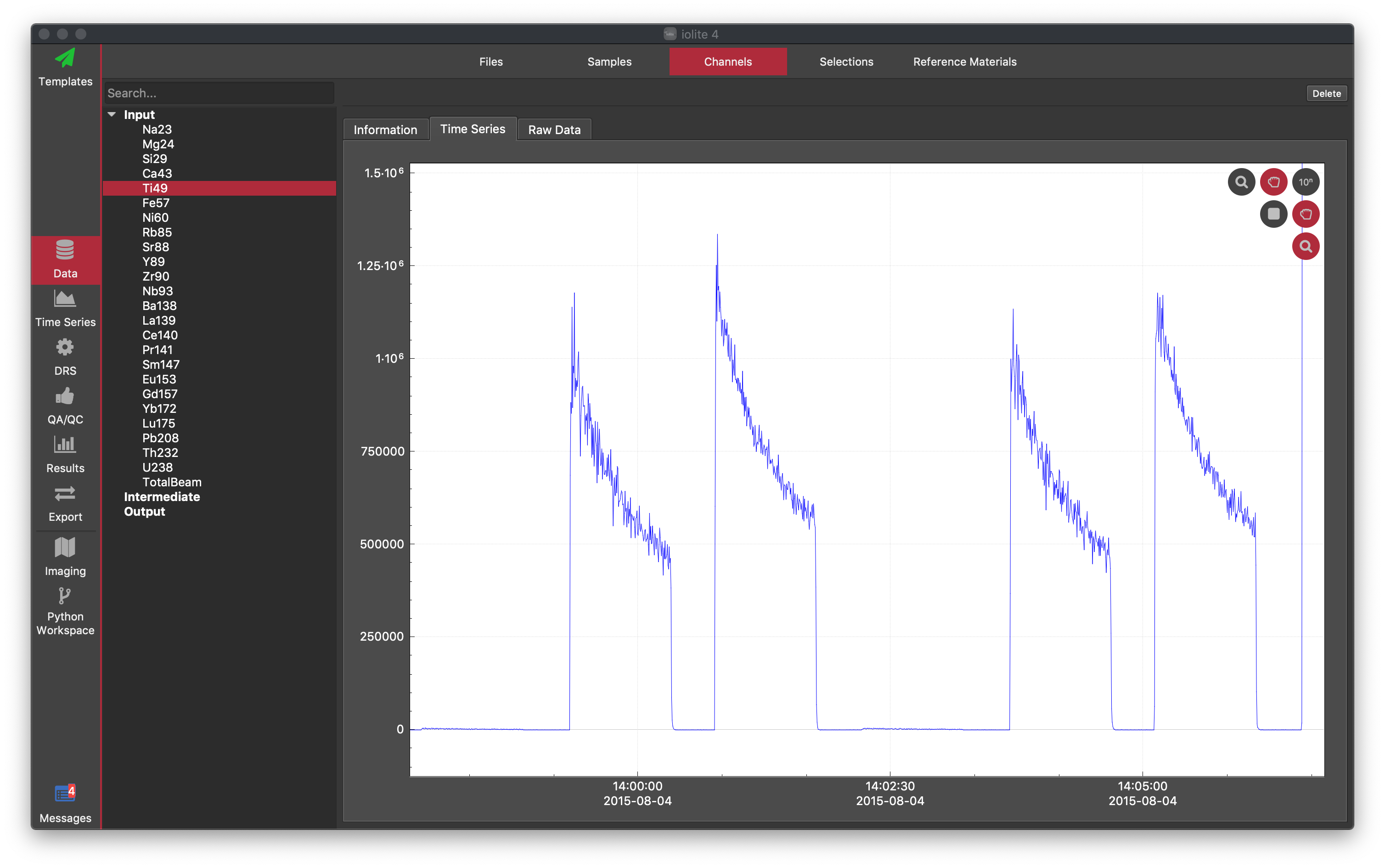
Time Series: This tab shows a graph of one or more channels vs time. Here you can adjust the x and y-axis scaling using the buttons at the top right of the graph. These are arranged in a horizontal and vertical sense. For example, the magnifying glass at the bottom enables zooming across the y-axis. To test this, click the magnifying glass at the bottom and then use the mouse-wheel to zoom in/out. You will see that you can zoom in the vertical direction whereas the horizontal direction is locked. If you also select the top magnifying glass, moving the mouse scroll-wheel will zoom in both the horizontal and vertical directions. Enable dragging by clicking any of the hand icons. In a similar way, each icon allows dragging in one direction. You can right click on the graph and select "Rescale" to reset the axis extents. Display the data in a log₁₀ scale by clicking "10ⁿ" button. Save the graph by right-clicking on the graph and selecting Save figure.
Raw Data: This tab shows the data for one or more channels in a table format. You can save the data within the table to either a .csv text file or .xslx Excel file by right-clicking on the table. Back to top

Selections Browser¶

The Selection browser displays information about a group of selections or individual selections.

The left-side window shows a list of selections grouped in three categories: Baselines, Reference Materials and Unknowns. With the exception of the Baselines group, any selection group that does not have a corresponding reference material file will be included in the Unknowns category. For example, if you have measured the reference material BIR-1G but do not have a reference material file for BIR-1G, the selection group will appear in the Unknowns group.

To see the selection groups within each category, click on the expand arrows. To see the selections within a group, click on the expand arrow beside the name of the group. Tip: To search for a particular selection, use the Search... box at the top of the list. The available information for a group or sample selection is displayed on the right-side window:

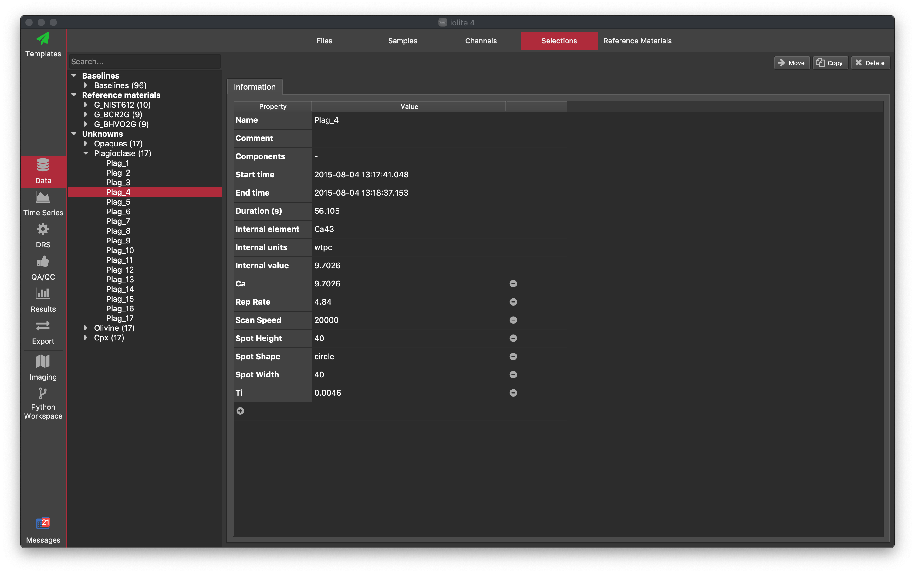
Click on a selection group's name to display information about the group and the selections within it.

Clicking on a selection within a group displays information about that particular selection.

Editing selections manually¶

Note

You can edit selection extents in the Time Series View LINK so that you can see the underlying channel data. However, you can also adjust the start and end times, along with other properties, of a selection here in the Selections Browser.

The Selection browser allows you to view and edit certain properties of all the selections within a selection group or of any individual sample selection at a time.

Editing Selection Group Properties:

You can adjust the following:

The selection group's name. It is not recommended to change the name of Reference Material group names (see changing group type below).
The selection group type (Baseline, Reference Material or Unknown). If you change your group type to Reference Material, the group name must match the name of a Reference Material exactly to be able to use its stored values.
Spline type: You can set the Spline Type for the group here. Setting the Spline Type for Unknown groups has no effect.
Duration: This sets the duration of every selection within a group by adjusting the selections end time. The start time for each selection will remain the same.
Internal Standard (IS) element/units/values: Here you can set the IS values for all selections within a group. For example, if you wanted to set all selections to use an IS value of 43.01 wt% Ca43, you would set the Internal element to Ca43, the Internal Units to "wtpc" and the Internal value to 43.01.

Editing Individual Selection Properties:

You can adjust the following for properties for individual selections:

The name of the selection

Hint

The name of a selection can be used to automatically assign internal standard values using the "Import IS values" button in the Trace Elements DRS, and via Processing Templates.

You can add a comment about the selection, such as anything that makes this selection different
Components: You cannot alter the components of a selection. Components are used in Linked Selections, and represent the individual selections that make up a Linked Selection.
Start and End time: You can manually enter the start and end time of a selection
Duration: you can enter the duration of the selection and the end time of the selection will be updated accordingly.
Internal Standard (IS) element/units/values: see the description above under Editing Selection Group Properties.
You can also add your own properties for a selection by clicking the grey icon at the bottom of the list of properties. This will add a new property called "My New Property" and will have a default value of "New Property Value". You can then double-click these values to change them. Using this feature you can add your own user-defined selection properties that can be used in custom QAQC modules, DRS, export scripts etc.

Move, copy or delete selections

Selections can be moved between groups, or copied to another group using the Move and Copy buttons at the top right. You can also delete selections by clicking the Delete button.

You can also drag and drop selections between the groups by selecting them in the list and dragging them to a new group. Back to top

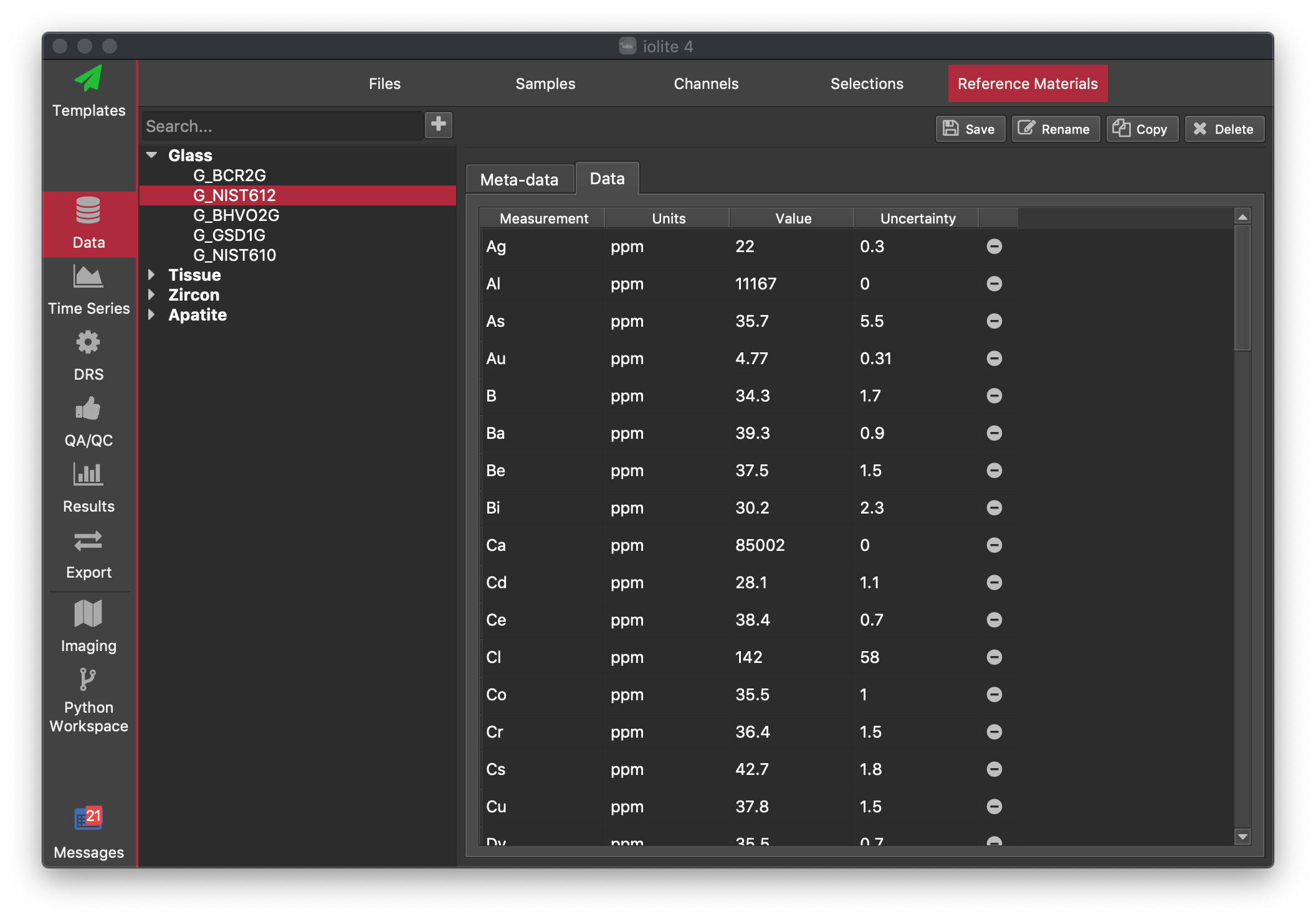
Reference Materials Browser¶

The Reference Materials browser shows the values and metadata associated with the available Reference Materials files.

Reference Material (RM) files are loaded at start up. To view or modify the folder iolite looks for RM files at start up go to Session -> Preferences (iolite4 > Preferences on Mac) or press Ctrl + , (Cmd + , on Mac) and select the Paths tab. The Reference Materials item will show the current location of the folder that iolite loads reference material files from.

RM data are stored in text files in JSON format (for more information about this file format, click here). Each RM file contains some metadata, such as the matrix type (e.g. glass, zircon etc), the data source (e.g. GEOREM), and a list of values in an array called "Results". See the default RM files included with iolite 4 for examples on how to create new files.

The Reference Materials browser is divided into two main parts: a list of RM that are grouped by matrix types on the left and the information area on the right. You can expand each of the listed group types by clicking the expand arrow. Clicking on any of the RM will display its information in the right-side window.

The right-side window has two tabs:

Meta-data: This tab displays information on the matrix type, data source, etc.
Data: This tab displays each of the values within the reference file. Values can be edited here by double-clicking on a value.

The default RM files included with iolite can be altered, but we strongly recommend that you create a new RM file by copying an existing one and editing that. You can copy an RM using the button at the top right.

You can remove a value by clicking the dash button to the right of the value. You can add a new value by clicking the plus button at the bottom of the list of values.

You can Copy/Rename/Delete RMs using the Copy/Rename/Delete buttons at the top right. Using the Save button will save a copy of the selected RM file.

Time Series View¶

The Time Series View allows you to view and modify the display attributes of the different channels. It also allows you to add and delete selections and selection groups, as well as to modify the duration of existing selections. It is called the Time Series View (TSV) because the data are displayed as a time series. To view the averages of selections, you can use the Results View **LINK**.

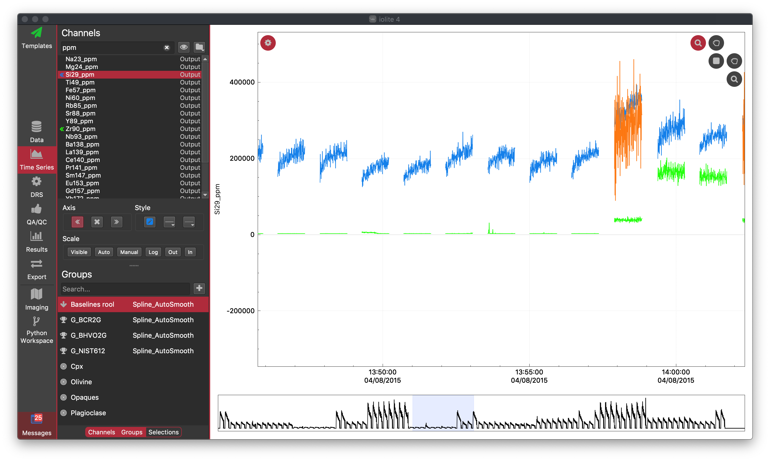
The TSV has two main components: the Settings Panel and the Time Series Plot. You can show/hide the Settings Panel by clicking the Settings Wheel icon found in the top-left corner of the Time Series Plot.

Settings Panel¶

The Settings panel is divided in three panes: Channels control, Groups display and Selections display. Each pane can be hidden or displayed at any time by clicking its corresponding toggle button at the bottom of the Settings Panel. In the figure above, the Selections display is not shown, and you can see that it is hidden because the Selections button at the very bottom is not selected.

Channel controls¶

This pane allows you to display and/or hide channels in the Time Series Plot. It also allows you to change the display attributes for each channel such as scale and style.

To Display A Channel:

Select a channel from the channel list. You can search to channels using the Search field at the top of the list of channels.

To add to the left axis you can double-click on the channel name, or you can click the button. To add the channel to the right axis, click the button. Note that the values of any channel are only displayed on the axis when selected in the channel list.

To Remove a channel from the plot, select it in the channel list, and click the button.

To Change the vertical scale:

Select a channel from the channel list.

Click any of the scale buttons found in the Scale control box to modify the scale of the y-axis of the selected channel on the Time Series Plot:

"Auto" autoscales the y-axis of the selected channel to fit the plotted data.

"Visible" resizes the y-axis of the selected channel to fit the extent of the data currently visible.

"Log" displays the y-axis on a logarithmic scale.

"Manual" allows you to manually supply the y-axis minimum and/or maximum for the selected channel.

"In" zooms in the y-axis of the selected channel.

"Out" zooms out the y-axis of the selected channel.

To Modify the Style:

Select a channel from the channel list.

Click any of the options found in the Style control box to customize the style attributes of the selected channel.

Clicking on the Pencil icon brings up the Color panel. This panel offers several color picker interfaces such as Color Wheel, Color Sliders, Color Palettes, Image Palettes and Crayons. How you choose a line color for the selected channel depends on the colour picker you select.

Use the Style button to change the line style. Channels can be drawn as solid, dashed, dotted and dash-dot lines.

The Weight button allows you to change the line thickness.

To Save Your Channel Display Setup:

You can add as many channels as you wish, and once you have set up your display, you can save the current channel settings to a setup file using the folder button at the top of the channels list. Here you can save or load channel settings to JSON files so that you can load them again in other experiments.

Hint

To limit the channel list to show only channels already added to the Time Series Plot, click the icon.

Groups view¶

This pane shows a list of all the existing selections groups. If the currently selected channel is plotted in the left y-axis of the Time Series graph, clicking on the name of a selection group displays all the existing selections for this group on top of the selected channel.

The list of groups has a symbol indicating what type of selection group it is: for baseline groups, for Reference Material groups, and for Unknown groups. Double-clicking on a group name will allow you to type a new name for the group. Note: you cannot change the name of a Reference Material group to a name that does not correspond to a loaded Reference Material name. For Baseline and Reference Material groups, you can double-click on the spline-type name to change the spline type for the group.

Right-clicking on a group name allows you to change the group type, or to remove a selection group.

To Manually Create a New Selection Group:

Click the icon next to the Search... field. The following window will appear.

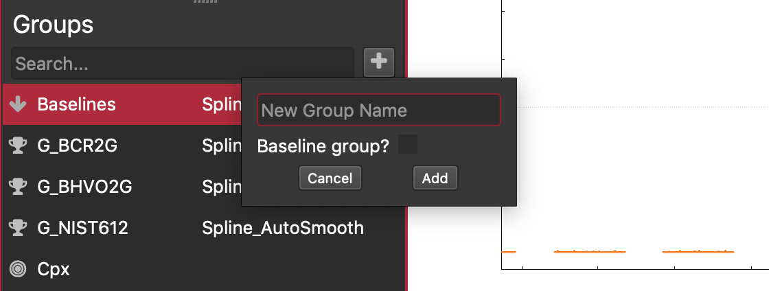
Enter your group's name. Reference Material group names must match the name of a loaded RM file exactly if you want to use the loaded RM values.
If you're adding a Baseline group, ensure you check the "Baseline Group" checkbox
Click "Add"

Selections display¶

This pane shows a list of all the selections in the currently selected selection group. Clicking on the name of a selection zooms in on that selection in the Time Series Plot.

Hint

You can use the Up and Down arrow keys to navigate the items in the list and inspect each selection. Note: You can also use the Search... input field at the top of the list to search for a specific selection. The search tools are case-sensitive and (for advanced users) does not use regular expressions such as | or *.

Selection Basics¶

Each selection is displayed as a rectangular box whose width and height represent the duration and 95% confidence limits, respectively.

If the box is bounded by a dashed red line, the selection is in Edit Mode and can be adjusted. You can only adjust the start and end points of a selection. The height and vertical position is determined by the underlying data.

If the box is bounded by an unbroken black line, the selection is not in Edit Mode, and cannot be adjusted. To return a selection to Edit Mode, hold Shift and left click on it. To exit Edit Mode, left click anywhere outside the selection interval.

To manually add a selection, select the group you wish to add it to in the Group List. Then hold down the Ctrl key (Cmd key on Mac) and left click and drag out the extent of the selection. The selection will initially be in Edit Mode until you click somewhere outside the duration of the selection.

To delete a selection, make sure that it is in Edit Mode (see above), and press the Backspace or Delete key.

You can delete all selections within a group by selecting one in Edit mode, holding Shift and pressing the Backspace or Delete key. You will be asked if you wish to delete all selections within the group.

When a selection is in Edit mode, you can press the 'a' key to show the selection properties:

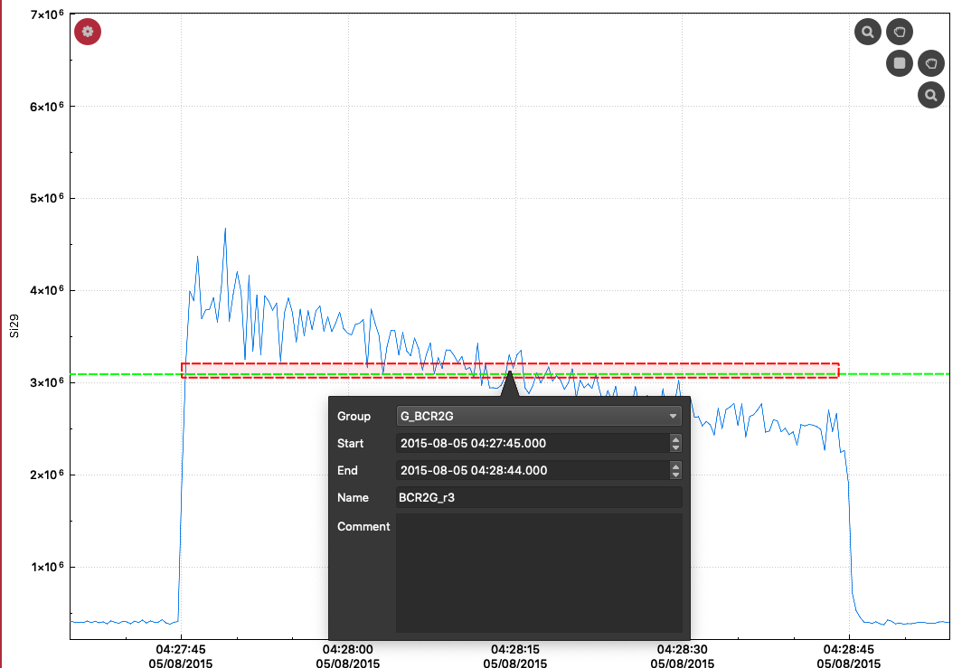
In the popup, you can adjust the start and end time, change the group that the selection belongs to, change the selections name and write comments about the selection. For example, you may want to make a note as to why you have avoided certain parts of the data to justify your selection etc.

Click elsewhere on the screen to close the selection properties popup.

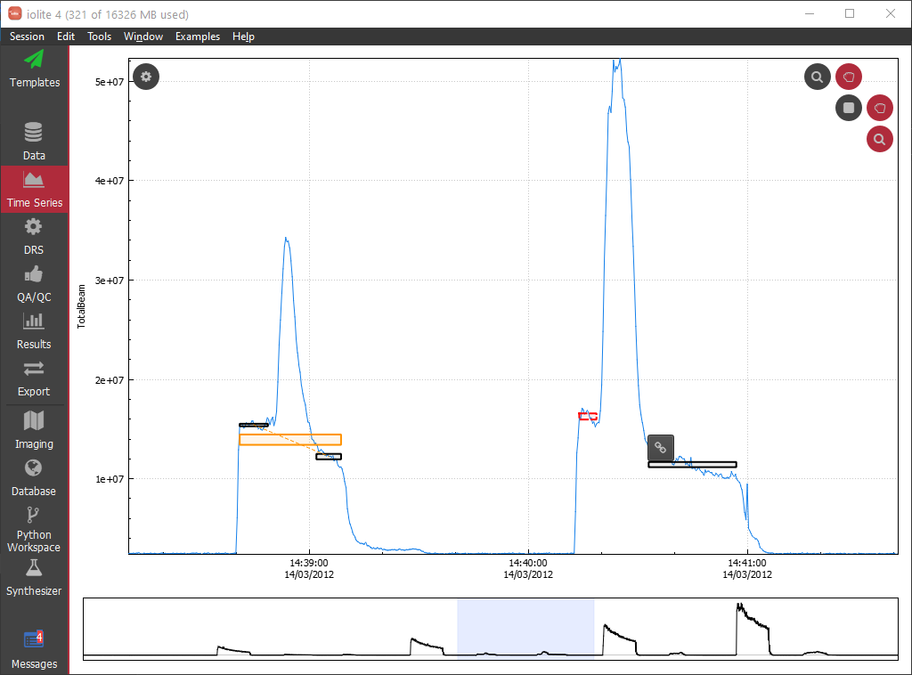
Linked Selections¶

In some cases, you may want to treat multiple selections as a single entity. For example, within a single ablation, there may be some sort of inclusion or spike that you want to omit, but still report only one result for the ablation. In this case, you'd use "linked selections". A linked selection is made up of multiple "component selections" (or subselections), and iolite will report the statistics such as mean, 2SE etc for the data that make up all of the component selections.

To link selections, Shift+left click on a selection that you want to link to enter Edit mode. Its bounding box will become a red dashed line. Then hover the mouse cursor over the selection you want to link. A small link icon will appear (see figure below). Click the Link icon, and the two selections are now linked.

A linked selection is distinguished from normal selections by its orange bounding box. Its component selections are linked by an orange dotted line. It is important to not overlap component selections. This would duplicate some of the measurements in the linked selection and make the statistics of the linked selection unrealistic. The vertical position of the linked selection is the mean of the data within in the component selections, and the left and right extents are the min and max of the component selection times, respectively.

You can un-link selections by shift+left clicking on a component selection, hovering the mouse over another component selection and clicking the unlink icon (it looks like a broken link).

An screenshot showing linked selections in iolite v4

If you create many sub selections, for example by using criteria that select only certain parts of your samples, you can automatically link them using a processing template action. Start with a blank processing template, add a 'Link Selections' action. Define which group contains the selections to be linked, and then set the maximum gap between selections. This gap determines which selections should be linked. For example, if your ablations are separated by 30 seconds of background measurement, set this value to 30. That way, any selections that are closer in time than 30 s will be linked, but the automatic action won't link together separate samples.

Time Series Window¶

The Time Series Window is divided into two sections: the main Time Series Plot and the Overview Widget at the bottom of the window.

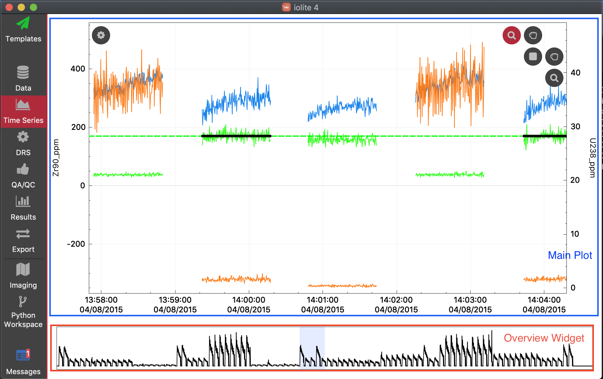
Overview Widget¶

This widget shows the entire extent of the currently loaded data, and displays Total Beam vs time. A blue rectangle highlights the current x-axis extents of the main Time Series Plot. Double clicking on this widget will autoscale the x-axis of the main Time Series Plot.

You can grab the left and right edges of the blue rectangle with the mouse and drag them to increase the x-axis extents manually. The mouse icon will change to a double-ended arrow when you are hovering over the edge. You can also click and drag the rectangle in the middle to move the axis extents left or right. The mouse icon will change to a hand when you can drag the blue rectangle.

Time Series Plot¶

The Time Series Plot displays time series data on a vertical axis versus time on the x-axis. Data can be plotted on the left or right axes.

Autoscaling axes

If you zoom in too far on the main window, you can easily rescale one or more axes:

To rescale the x-axis, right-click on the plot and select Rescale. Alternatively, you can double-click on the Overview Widget at the bottom of the window.

For detailed scaling of the y-axis, see the Channel controls above.

Graph controls

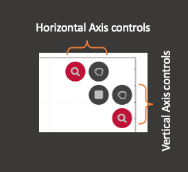
There are five buttons in the top right corner of the Time Series Plot. There are two zoom tools. If the vertical zoom tool is 'on' scrolling the mouse wheel will zoom in/out the vertical axis for the currently selected channel. You can turn each zoom tool 'on' or 'off' by clicking the icon. If the horizontal zoom tool is on scrolling the mouse wheel will zoom the x-axis in and out. If both are on, scrolling the mouse wheel will zoom both axes. If neither are on, nothing happens when you scroll the mouse wheel.

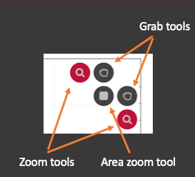
The iolite Main Time Series Plot control labels

There are also two grab tools: one for dragging the vertical extent of the graph and another for dragging horizontal extents. They are turned on and off in the same way as the zoom tools. If the vertical grab tool is turned on, clicking on the main plot with the left mouse button and dragging will move the vertical extent of the plot (while maintaining the current level of zoom). The horizontal grab tool acts in the same way. If both are turned on, you can drag both horizontally and vertically at the same time.

The iolite Main Time Series Plot control arrangement

There is also an area zoom tool. Turning this tool on will allow you to drag out an area using the mouse. Whether the vertical or horizontal axis (or both) is zoomed depends on which zoom tools are turned on. The grab tools are not compatible with the area zoom tool and their icons are not shown while the area zoom tool is active.

Tip

You can drag the plot to the Notes panel (*LINK TO NOTES PANEL*) to save a copy of the current plot in your Session Notes. Using this you can write notes about interesting observations about channel results for each group etc.

You can show information about a particular selection, such as the start and end times, the selection label, and any comments associated with the selection, by shift+clicking on a selection (or by selecting it from the list of selections in the Selections section of the Setup Panel) and pressing the 'a' key. This will show a small dialog that shows information about the current selection.

Hover Stats Plugin¶

If you would like to see the mean value for each selection while still viewing the Time Series data, similar to the Sample Info panel in iolite v3, you can open the Hover Stats window (Tools menu -> Hover Stats). This will pop open a window that always remains on top so that you can see the average value (and error bars) for an uncertainty while adjusting it in the Time Series window. This panel can be open with any View open in iolite v4 (not necessarily the Time Series View).

Data Reduction Scheme (DRS) View¶

The DRS View allows you to select a DRS. A DRS is the code that calculates your final results from your raw data. Typically they include steps such as baseline subtraction, normalisation to a reference material etc. A DRS can be run multiple times. Each DRS requires some information to be able to calculate all the results. For example, to do baselines subtraction you must have selected some baseline selections. However, if you have not provided all the information needed, the DRS will do only what it can with what you have provided and stop. For example, if you have selected baselines, but no reference materials, and run the Trace Elements DRS, it will perform the baseline subtraction, and normalise each channel to the internal standard (if using an internal standard), and then stop because there are no reference material selections. You can view the channels that have been calculated up to that point, and any results associated with it, but the DRS will not be listed as "finished". Once a DRS has finished, it will then update all the results (Results View Link).

You can apply more than one DRS to a dataset/session. For example, for the same session, you may want to calculate trace element concentrations using the Trace Elements DRS and U-Pb ratios using the U-Pb Geochronology DRS. You can just run each DRS in turn.

From the DRS browser, you can select the DRS that will be applied to the data by clicking one of the items in the list on the left side of the window. The settings options corresponding to the selected DRS are displayed on the right side window.

By default there are four DRS available in the current version: Baseline Subtract, Hf Isotopes, Trace Elements, and U-Pb Geochronology, each of which is briefly described below.

Index channels¶

Most DRS require an "Index Channel". An index channel is an analyte that is present in every analysis. Because iolite allows flexibility during data import, not every channel must be present in all imported files. However, the index channel must be present throughout the entire analysis to allow the creation of an "index time" reference. The index time is a direct copy of the Index Channel's time data, and will include any gaps in acquisition, it is therefore important to select a channel (mass) that has been acquired for all analyses. Index Time is then used as the time wave for any splines etc created when a DRS is run.

If data have been acquired simultaneously from multiple machines it is recommended to select an Index Channel from the machine with the highest sampling frequency to minimize down-sampling of input data. This may have implications for the number of points for a given channel (i.e. resampling may increase the number of points in a selection).

Masking¶

Masking is a common task in DRS. The concept is to "hide" or mask all baseline intervals. The reason for this is that if you have a DRS that calculates ratios, the backgrounds will have a very large range (dividing by a very small number will create a very large number). This large range will make the range of your samples appear very limited and you won't be able to see much information (without zooming in significantly). There are two options for masking: using the laser log file and using a threshold.

Using the Laser log method will simply blank out any values that do not correspond with a laser on event recorded in the loaded laser log files. Not that the Mask channel and Mask threshold values are ignored if using the laser log method.

The Cutoff method works by blanking out all values below a certain threshold. Whenever the Mask Channel is below the threshold, all intermediate and output channels will be blanked out.

Note

Input channels are never altered by any DRS, which is why you can re-run your DRS as many times as you like, and run multiple DRS on the same input data.

There is also a Trim option which will trim off an addition amount time before and after the threshold has been passed (or before or after the laser switches on/off if using the laser log method). For example, if the Cutoff is set to 1000 CPS, and the mask channel is Ca43, and the Trim value is set to 1 s, any time the Ca43 channel drops below 1000 CPS all datapoints for intermediate and output channels will be blanked out. An additional one second worth of datapoints will also be blanked out due to the trim value at the start and end of these intervals.

If you are seeing intervals with no data where you expect sample data to be, it could be that your mask threshold is set too high. We recommend that you turn masking off, and re-run your DRS to see if this fixes the problem.

Hint

One other way that you may see the blank intervals where you expect sample data is when using internal standards and the Trace Elements DRS. If there is no IS value for an interval, output channels can be calculated (because they rely on the internal standard value in the calculation).

You can get more information about masking in this iolite note.

To create masks from the python API, please see this part of the API documentation.

Baseline Subtract DRS¶

This DRS allows you to perform a basic background subtraction on the data. See above for a discussion of Index Channels and Masking.

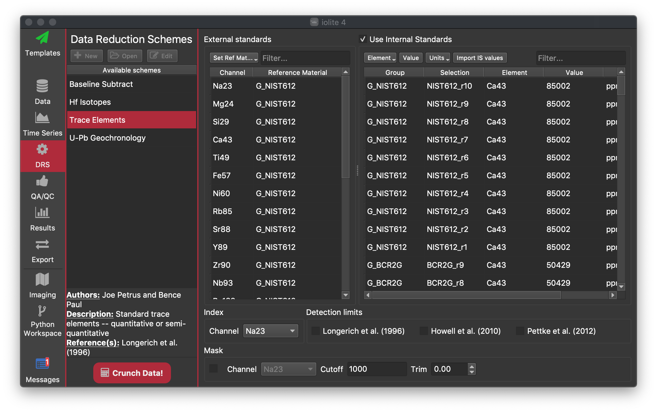
Trace Elements DRS¶

The Trace Elements DRS calculates trace element concentrations using established methods which include background subtraction and normalisation to an external standard, and depending on the user settings may include normalisation to an internal standard.

The Trace Elements settings window is divided into five main parts:

External standards¶

iolite uses the sample-standard bracketing approach for external standardisation. This type of normalisation allows for the correction of instrumental drift over an experimental session by reference to standards measured in the same session. A major advantage of the Trace Elements DRS is that it supports the use of different reference materials for external standardisation of each analyte. This is useful when, for example, your primary reference material does not include all the measured analytes or when the abundance of a particular analyte has been better characterised in a reference material other than your primary standard.

The External standards settings box allows you to define the reference materials that will be used for external normalisation, as explained below:

Select one or more channels from the Channel list. The selected channels will be highlighted in red. You can select all channels with Ctrl + a (Cmd + a on Mac).
Choose a reference material to be used with the selected channels from the 'Set Ref Mat...' drop-down menu found at the top of the table. The selected reference material will be listed in the Reference Material list, next to the corresponding analyte.

Hint

If you want to select a reference material for a single analyte, you can double-click on the 'Reference Material' field next to the analyte's name (highlighted in blue) to prompt a drop-down menu containing all the reference materials available for selection.

Internal standards¶

The Internal standards settings box allows you to specify whether to use an internal standard element (IS) for the quantification of trace elements concentrations or perform a semi-quantitative analysis. Check the 'Use Internal Standards' check box to enable internal standardisation or deselect to enable semi-quant mode. When you choose to work in semi-quant mode, the Internal standards settings box is disabled and no changes can be made.

Follow these steps to set up internal standardisation:

Select one or more selections from the sample list. You can use the Search... field at the top to search by selection name. You can press Ctrl + a (Cmd + a on Mac) to select all selections (quite useful when using the same IS for all selections).
Select a channel from the Element drop-down menu found at the top of the list corresponding to your Int Std (e.g. select Ca43 if using Ca as the internal standard).
If any of the selected selections belong to a reference material, the corresponding reference concentration and concentration units will be automatically filled in the table from the reference material files.
You can input the IS concentration value for each sample by clicking on the corresponding Value field and entering the value using the keyboard. To input the same IS concentration value for multiple sample selections, first select the samples from the list and then click on the Value button found at the top of the list.

Hint

You can copy and paste from/to this table using Ctrl+c/Ctrl+v (Cmd+c/Cmd+v on Mac). For example, you can copy out all the selection names into an Excel spreadsheet, arrange all the IS values in the correct order, and then paste these values into the table in iolite.

Make sure to choose the correct concentration units. You can change the units for an individual selection by double clicking on the Units field and choosing the correct option from the drop-down menu. To change the the units of multiple selections use the Units drop-down menu found at the top of the table.

If you have IS data stored in a comma-separated values text file (.csv) or in a delimited text file (.txt), you can import the data by clicking Import IS values at the top of the IS table. For a successful import, the file must include information on sample (selection) name, element and concentration. The table should be configured in the following format: * the first row contains the headers (e.g. SampName (tab) Ca (tab) Ti)) * the first column contains the sample names. iolite matches the sample name information in the file with the names of existing selections. If the names do not match, the selection will not receive the IS values.

*LINK: See the Gabbros trace element example for an example IS values file *

Index channel¶

See above for a discussion on index channels.

Detection limits¶

The Detection limits option allows you to specify the approach that will be used to determine the limits of detection (LOD). Check the corresponding check box to calculate any of the three available methods: Longerich, Howell or Pettke.

Longerich et al. (1996) [1]

Here the limits of detection are defined as:

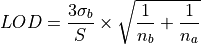
$LOD = \frac{3\sigma_{b}}{S} \times \sqrt{\frac{1}{n_{b}} + \frac{1}{n_{a}}}$

where the $LOD$ is the limit of detection for the element,

$\sigma_{b}$ is 1 standard deviation of the background measurement for this element,

$n_{b}$ is the number of measurements in the background selections (e.g. number of sweeps in the background measurement, for a 60 s background measurement: 60 s times 2 sweeps per second = 120 background measurements),

$n_{a}$ is the number of measurements in the sample selection (as for backgrounds), and

$S$ is the sensitivity (e.g., CPS/ppm). Sensitivity is calculated by:

$S = \frac{R_{ancal}} {C_{ancal}} \biggl[ \frac {R_{ISsam}} {R_{IScal}} \frac {C_{IScal}} {C_{ISsam}} \biggr]$

where $R_{ancal}$ is the count rate of the analyte (e.g. 88Sr) in the calibration standard (e.g., NIST612), usually in CPS,

$C_{ancal}$ is the concentration of the analyte in the calibration standard,

$R_{ISsam}$ is the count rate of the internal standard (IS) isotope (e.g. 43Ca) in the sample,

$R_{IScal}$ is the count rate of the IS in the calibration standard,

$C_{IScal}$ is the concentration of the IS in the calibration standard, and

$C_{ISsam}$ is the concentration of the IS in the sample.

One downside of this method is that it will produce an LOD value of 0 for channels that have no variation in their baselines (e.g. a baseline that is all zeroes except when the laser is on). This may mistakenly suggest that the limits of detection are infinitely low, which in turn renders any counts detected by the mass spectrometer significant. To avoid these falsely significant results, the Howell and Pettke methods described below provide alternative approaches for estimating LOD at low counts levels.

Howell et al. (2010) [2] :

This method replaces average background variation values (i.e., standard deviation of the background measurement) of zero counts per second with 7. The value of 7 CPS represents the number of counts required to be 3.3σ (i.e, 99.9% confidence interval) above a background signal of 0 counts.

Pettke et al. (2012) [3] :

This method (Pettke et al., 2012) uses an approximation to Poisson distribution statistics for estimating LOD, which takes into consideration the uncertainty at low count rates. Here LOD (in µg.g^-1) is defined as:

$LOD = \frac {3.29 + \sqrt{ R_{bkg,i} \times DT_{i} \times N_{an} \times (1 + \frac {N_{an}} {N_{bkg}} ) } + 2.71 } {N_{an} \times DT_{i} \times S_{i}}$

where $R_{bkg,i}$ is the mean background count rate (in CPS),

$DT_{i}$ is the dwell time for the given isotope (in seconds),

$N_{an}$ and $N_{bkg}$ is the number the number of sweeps for the analyte and background measurements (sweeps), respectively, and

$S_{i}$ is the sensitivity of element $i$ (in CPS per µg.g^-1).

The coefficient 2.71 is associated with the 5% probability (i.e, 95% confidence interval of the Poisson distribution) that no counts will be detected during acquisition at very low count rates.

Note

For $R_{bkg,i}$ , $\sigma_{b}$ , $n_{b}$ and $N_{bkg}$ in the above equations, iolite finds the closest baseline selection and used the values from that selection in the calculation.

U-Pb Geochronology DRS¶

The U-Pb Geochronology DRS calculates U-(Th)-Pb ratios for geochronology with downhole fractionation for U-Pb and Th-Pb ratios. It is based on the method outlined in Paton et al [4]

The U-Pb Geochronology settings window is divided into four main parts:

Basics¶

Index Channel: see above for a discussion of index channels

Reference Material: Analyses of this reference material will be used to construct the downhole fractionation model, and to correct for elemental bias in the downhole corrected ratios.

Default fit type: This is the model to use for the downhole fractionation correction. For example, if the observed downhole fractionation in your reference material appears to be linear, you would select the "Linear" option in this list. The actual evolution of the ²³⁸U/²⁰⁶Pb ratio with time (i.e. the downhole fractionation) is a product of several factors including cell design, gas flows and others. We refer you to the literature for the causes of downhole fractionation. While we cannot advise on the best model for your analytical setup, the best test of how well a correction has worked is to view the final ratios (e.g. Final206Pb238U) to see if there is any residual trend in the data (the overall pattern should be flat). One good way to view all selections for a group at once is to use the Tools -> Stacked Plot window. This plots the results for every selection within a group with their start times aligned. Looking at all the selections in this way can reveal trends not obvious looking at a single selection.

Beam Seconds¶

Downhole fractionation is due to the effect of drilling a hole into your sample, and fractionation increases with depth. As we do not have a direct measurement of each ablation pit's depth, we need to use time as a proxy for depth. This is where Beam Seconds comes in. It is how long the laser beam has been ablating the sample. Before laser log files were common, when the laser started firing had to be inferred from the measured signal. However, this has several drawbacks and we recommend recording and using a laser log file whenever possible (*LINK TO LASER LOG FILES SECTION*). Setting the Beam Seconds method to Laser log file will use the laser log to determine when the laser started firing and this will be used to create the downhole fractionation graphs (e.g. 206Pb/238U vs Beam_Seconds).

Jump Threshold

Using this method, a smoothed (5-point box smooth) copy of the index channel is created and then each time the difference between measurements is greater than the Beam Seconds sensitivity, it is recorded as a laser on/off event. This is in effect looking at the gradient of the Index Channel and each time the absolute gradient exceeds the threshold, it begins counting again from 0 s.

Cutoff Threshold

This is similar to Jump Threshold except that it uses the counts of the index channel (instead of the gradient). Whenever the counts of the index channel exceed the threshold set in Beam Seconds sensitivity, it begins counting again from 0 s.

Gaps between Samples:

This method uses the sample information from the imported mass spectrometer data files (you can see these samples in the Samples Browser **LINK TO SAMPLES BROWSER**). Each time a sample starts, beam seconds starts at 0 and increments until the end of the sample. This is the recommended method if you do not have a laser log file and your mass spectrometer records each sample in its export file (e.g. X-Series files).

See above for a description of Masking

Other Parameters¶

Here you can set the ^{238`U/:sup:`235}U ratio and the decay constants for each parent isotope.

For a more detailed description of the U-Pb Geochronology DRS, see ****the U-Pb Geochronology DRS tutorial.*****

QAQC View¶

The QAQC View shows QAQC (Quality Assurance/Quality Control) data and reports. QAQC results are calculated and visualised by QAQC modules. iolite v4 comes with two basic QAQC modules: ElementCheck and SecondaryCheck.

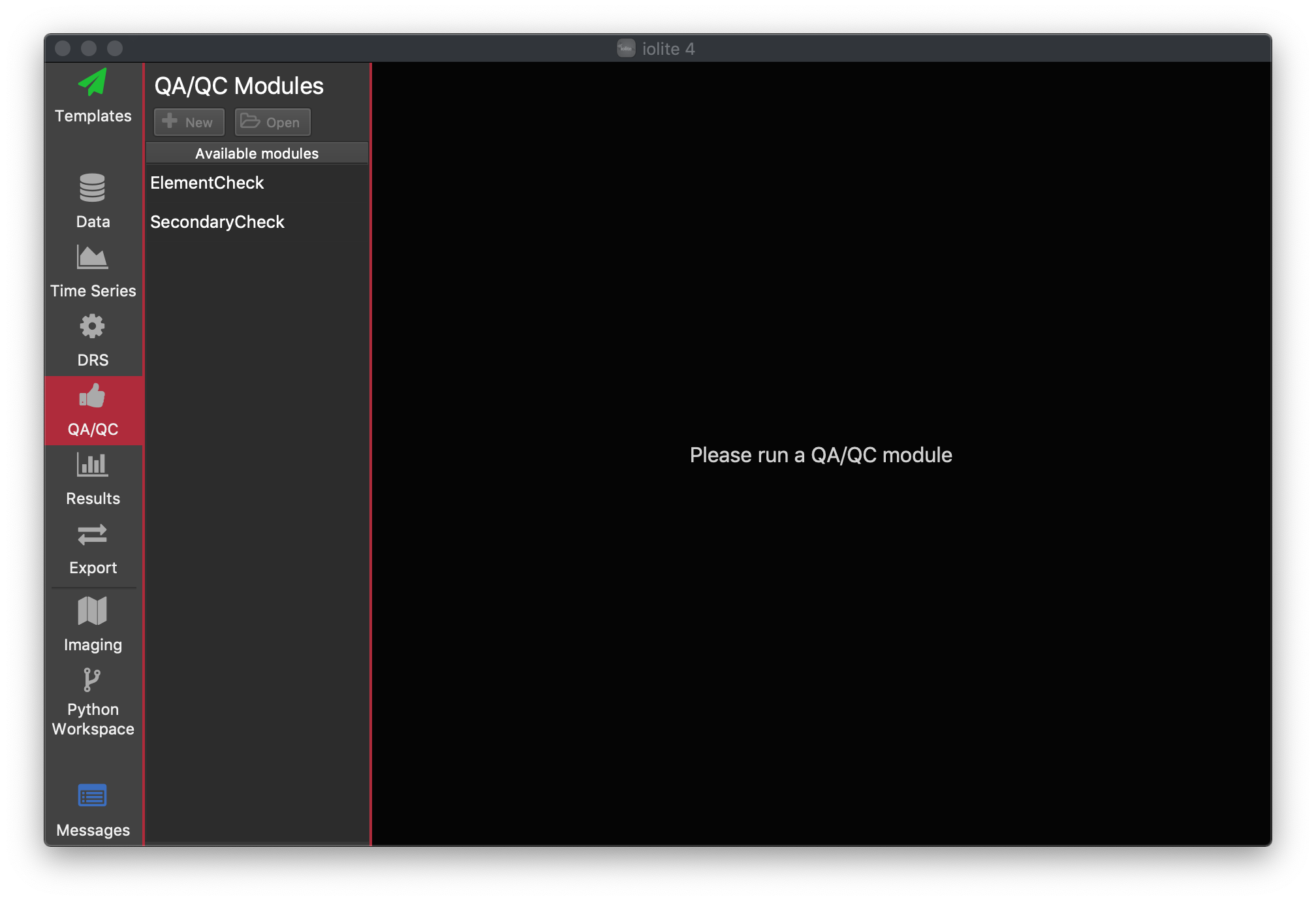
You can select a module on the list on the left hand side, and double click it to run it, or select it and click the Run Module button at the bottom of the list.

Each module opens as a new window on the right hand side of the window. You can multiple instances of each module running. You can minimise, maximise, restore down and close each modules window using the buttons at the top right of the module window (just like a Microsoft Windows window). We recommend maximising the module window when you first open a new module to see all settings and results.

Python QAQC modules can be created by clicking the +New button at the top of the module list, and existing python QAQC modules can be opened using the Open button.

Each QAQC module usually has a Settings button and Run button at the top left of the module window. Most will also have an Export button at the top right of the module window. See the figure below for an example.

QAQC results can also be saved at export time (*LINK TO EXPORT VIEW*). If exporting to an Excel file, QAQC results can be included in the exported file in their own worksheet. If exporting to a text file, the QAQC table will be saved to a text file, and plots are saved as png files.

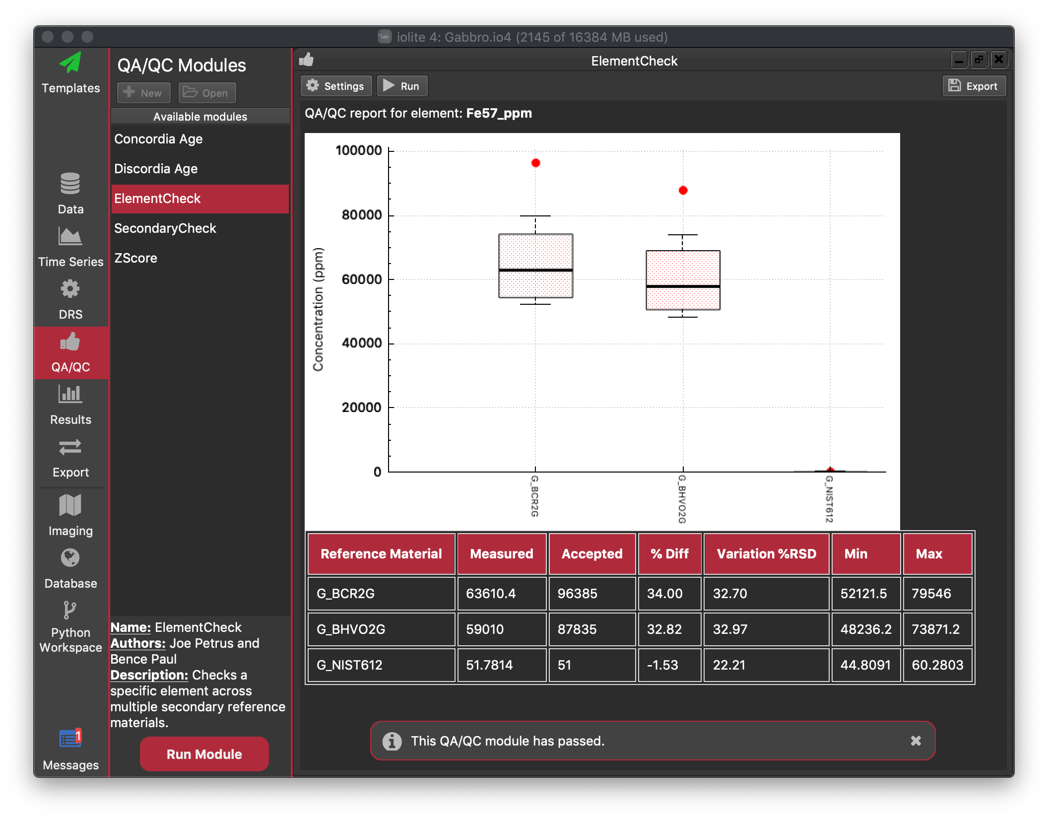
ElementCheck QAQC Module¶

This module presents the QAQC results for a single element at a time. You can select the element of interest using the Settings button in the top. The module will present the accepted value for each Reference Material along with some statistics for the measured values in the current experiment. In the table of results (below the plot) the measured value, accepted value and percentage difference (% Diff) are reported. Here the measured value is the mean of the selections within the selection group (with no outlier rejection). The variation within the group, presented as % RSD, calculated by $100 \times \frac {groupUncertainty} {groupMean}$ , is also reported, along with the minimum and maximum values for the group.

In the plot, the accepted value is plotted as a red circle. The results for each group are plotted as a statistical box plot (see example above). The variation in each group may be so low that you cannot properly see the box for each group (where the uncertainty within each group is much less than the variation between groups). More information about statistical box plots is available here, but briefly the bottom and top lines defining the red region are the 25th Percentile (aka the first quartile, $q1$ ) and 75th Percentile (aka the third quartile, $q3$ ), respectively. The median value is represented by a solid black line through this box. The whiskers above and below the interquartile range ("iqr"; $q3 - q1$ ) show the maximum and minimum values. Outliers (defined here as values greater than $q3 + 1.5 \times iqr$ or less than 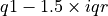$q1 - 1.5 \times iqr$ ) are plotted as blue unfilled circles, if any exist.

Note

Although results for the primary reference material will be included in the QAQC results, they will always be within a few percent of the true value (depending on your chosen spline type: experiment with different spline types to see this effect), so you should not put much stock in these results. Secondary reference materials are always the best indicator of data quality, and the more that you measure, the better you can guage the quality of your results.

Clicking the Export button (top right of module window) will save a html version of the plot and results table. You will be prompted for a location for the exported file.

Note

The "Run" button in this QAQC module does nothing as the module automatically runs each time you change the channel of interest. For larger modules, where there are more settings and the module may take quite a while to run, the Run button is clicked to signal the the user is ready to recalculate the results.

SecondaryCheck QAQC Module¶

This module presents details QAQC results for a selected secondary reference material. The mean of all selections within the ref mat group are compared with the accepted value (taken from the ref mat file) to calculate a percentage difference (% Diff). The QAQC results comprise a plot of the percentage difference for each channel measured, and a table including the percentage difference, as well as the relative variation (calculated by $100 \times \frac {groupUncertainty} {groupMean}$ ), and minimum and maximum results for selections within the group.

Results are coloured according to Alarm and Warning levels: if a value does not exceed the Warning or Alarm value, it is shown in black. However, the user can set an Alarm level, where if a value exceeds this absolute difference from the accepted value, an error will be listed in the Messages View (*LINK TO MESSAGES VIEW*). Additionally, if the QAQC module is running as part of a Processing Template, the user can opt to have the Processing Template halt on the raising of an alarm (this stops the rest of the template running if there is an issue with the results, which is what QAQC is designed to determine). Values that exceed the Alarm value are shown in red in the table of results (to highlight that an error has occurred).

Similar to an Alarm is the Warning level. If the mean value for an element exceeds this absolute difference from the accepted value, but is less than the Alarm value, a Warning will be raised. However, unlike an Alarm, a warning is just logged in the Messages view and any Processing Template will not be halted. This is designed to only alert the analyst that there may be issues with this channel. Values that fall within the range of a warning (that is Warning Value < mean result < Alarm Value) are colored yellow in the results table.

The default Warning and Alarm values are shown as dashed and solid red lines, respectively, in the results plot.

Similarly, the analyst can set Warning and Alarm values for variation within a group. Excessive variation may indicate some instability in results, even if the mean is within the acceptable value relative to the accepted value.

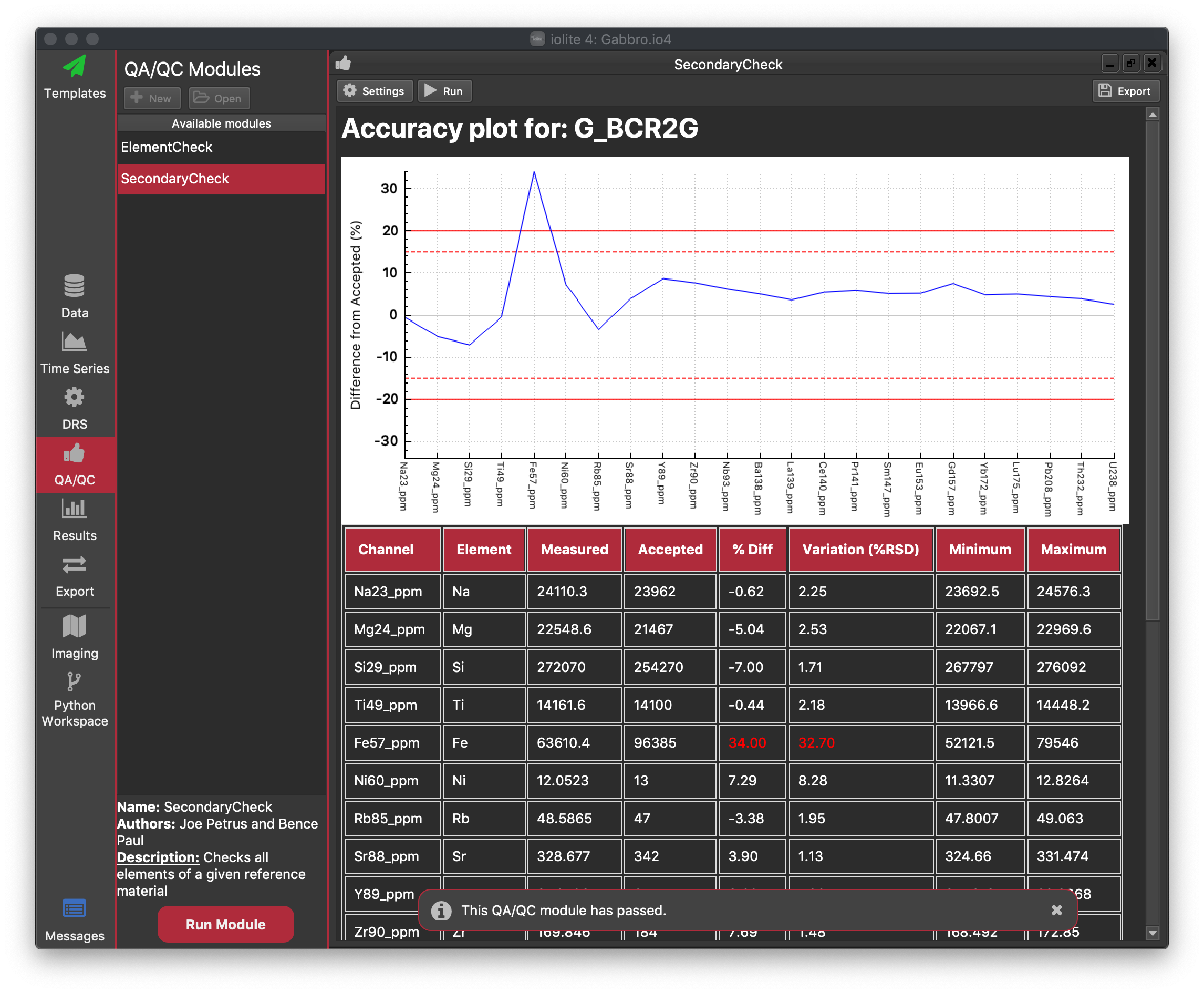
The default Alarm and Warning values (for both percentage difference from the accepted value and for group varation) can be set in the Settings menu for this QAQC module.

In addition to setting the default value (which is applied to all channels), "exceptions" can be defined, which are Warning and Alarm values for individual channels. For example, if a channel has a poorly calibrated value in your reference material file, or if you expect that a channel will vary widely but do not want it to raise an Alarm and potentially halt the Processing Template, you can create an exception for that channel with a larger % Diff value or Variation value. In the figure above, an exception has been set for Fe in the current experiment so that an Alarm will not be raised.

You can save and load settings for Alarms, Warnings and Exceptions using the button at the top right of the Settings panel.

Clicking the Export button will save the current report to a html file, which includes both the plot and table.

Results View¶

The Results View shows selection- and group-level results (in contrast with the Time Series View, which shows results without any averaging and in time-series). There are three tabs: the Summary Stats Tab, the XY Plot Tab, and the Data Table tab, similar to the same tabs in iolite v3.

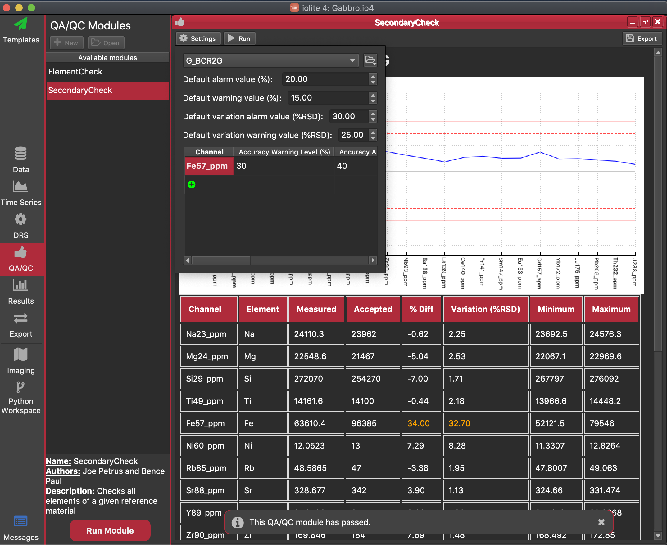
Summary Stats Tab¶

This tab shows the mean and uncertainty for each group for the selected channel in table form in the top third of the screen, and mean and uncertainty, along with the result for each selection within the group, plotted in the lower two-thirds of the window. To add a group to the plot check the checkbox to the left of the group's name in the table. Multiple groups can be added to plots at once.

The selected channel can be set using the controls at the top right, along with variations on how the mean is calculated, the expression of variation within the group (e.g. 2SE, 2SD etc), and whether outlier rejection is performed in the mean/uncertainty caculations. Note that changing the uncertainty as expressed as an absolute value, percentage value, or ppm value does not affect the plot as it is the same value, just expressed differently. This does however affect the value shown in the Uncertainty column of the table.

In the plot, a mean value for each selection is shown, along with error bars showing 2SE for the selection. Selections are orderded by start time. Hovering the mouse over any selection will show more information about that selection, including the selection name, start and end time, mean, uncertainty and number of outliers.

Tip

Double-clicking on a selection in this plot will pop up a panel showing the underlying time-series data for this channel and the selection extents. You can edit the selection start and end times right here in this window, and the selection extents will be updated for all channels. This can be handy to see if a selection is abnormally high due to an inclusion in the current analysis. Clicking the button will zoom the Time Series View plot to the current selection. Clicking the 10ⁿ button will change the vertical axis between log and linear scaling.

You can manually set the color of each group by double-clicking its color in the Groups summary table (in the top third of the window). You can also assign random colors to each group using the "Assign Random Colors" on the right.

Tip

You can drag the plot to the Notes panel (*LINK TO NOTES PANEL*) to save a copy of the current plot in your Session Notes. Using this you can write notes about interesting observations about channel results for each group etc.

XY Plot Tab¶

The XY Plot is set up the same as the Summary Stats Tab (see above), with a table of group results at the top and a plot in the lower two-thirds of the window, except that here you can plot the results of one channel against another. This can be useful when looking for correlations between channels, or trying to identify outlier selections in more than one channel. The plot controls in the top right of the plot are the same as for the Time Series Window in the Time Series View (*LINK*).

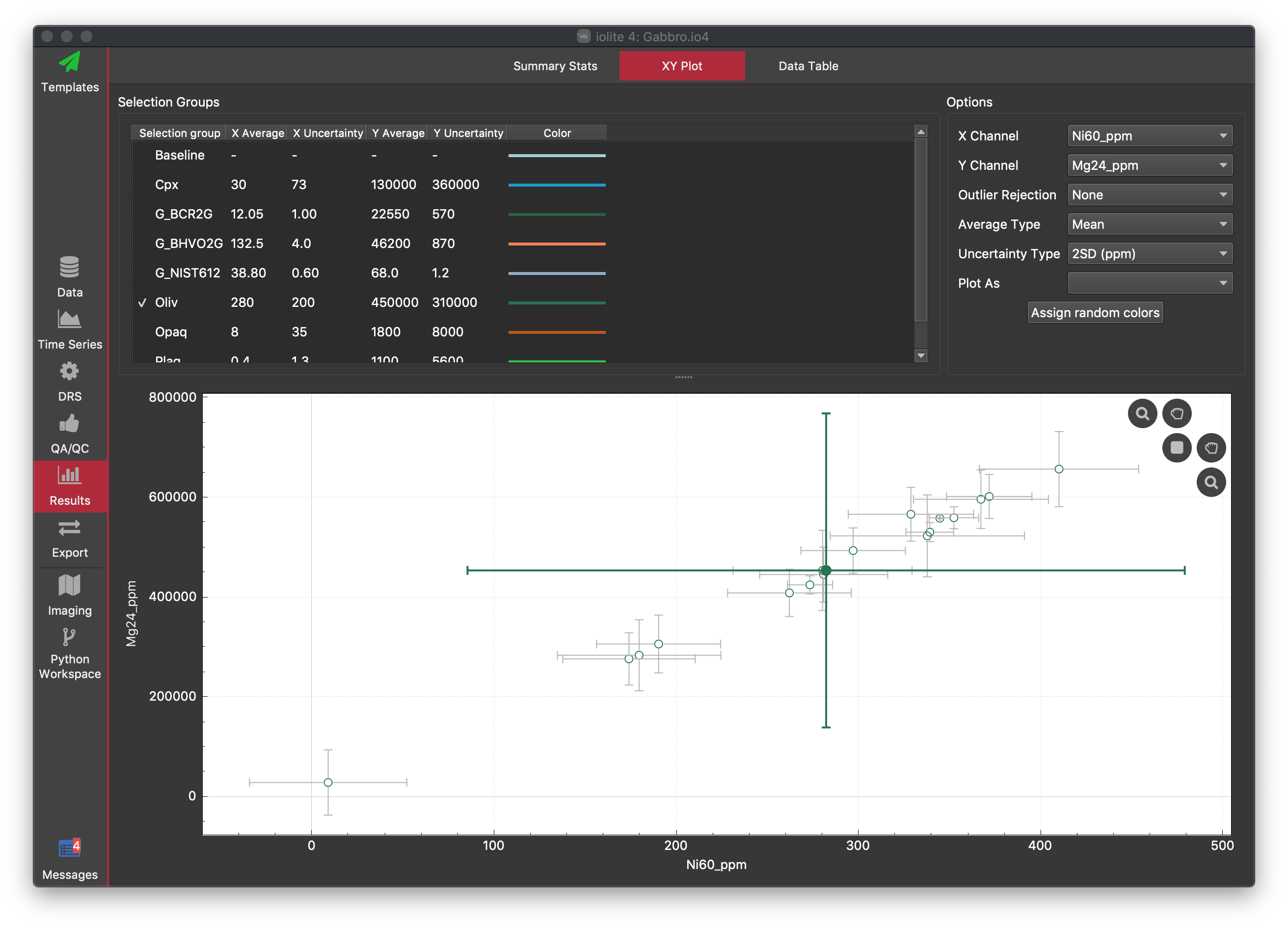
In the XY Plot, the mean for the group is shown as the larger filled symbol, and results for each selection within the group are shown as unfilled circles.

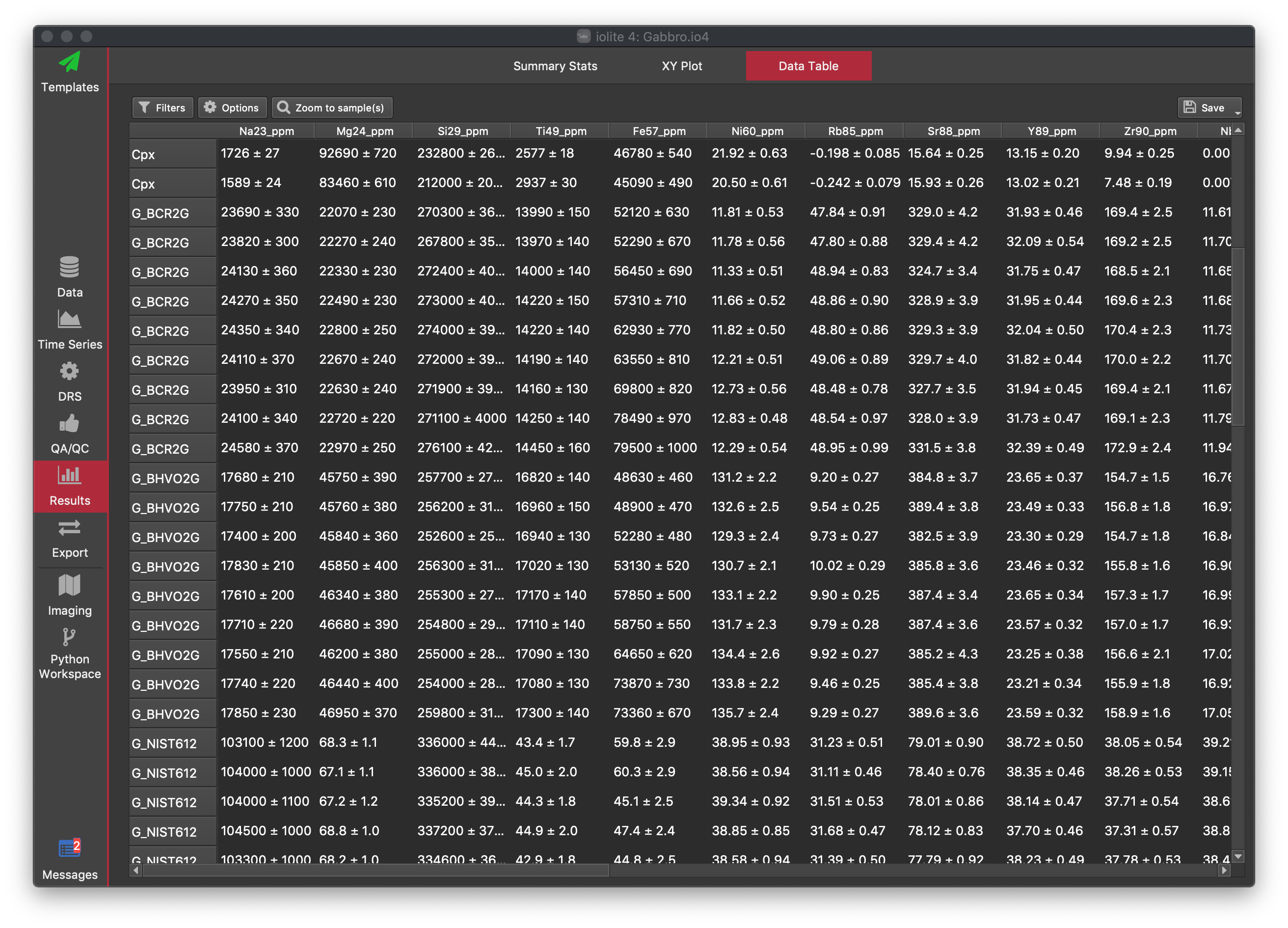
Data Table Tab¶

The Data Table tab shows results for each selection in a table format. The selections that are shown, and the columns that results are shown for can be adjusted by the user to display the information the analyst is most interested in. By default, all selections and columns are shown. There are columns for selection metadata (e.g. spot height, comment etc), and one column for each input, intermediate and output channel. If a column is represents a channel, the values in the column start by showing the mean ± the uncertainty (2SE), but Limits of Detection (LOD) values can also be shown.

The channels, selections and values shown can be adjusted using the Options button (for common operations) and the Filters button (for customised filters).

Options Panel¶

At the top of the options panel (opened by clicking the Options button ), you can select what type of channels (input, intermediate or output) channels you want to include in the table by clicking the checkbox next to each category name. Similarly, you can select which selection group types you want to show (Baseline, Reference Material, or Samples) by checking or unchecking the checkboxes each group type. Uncertainties can be shown/hidden by checking/unchecking the Errors checkbox. If errors are shown, you can select what level of uncertainty you wish to show: basic (the 2SE for data within the selection interval, with/without outlier rejection), propagated (if you have run a DRS with propagated errors and have run sufficient reference materials etc), or RMInc (a propagated uncertainty with uncertainties from the values in the reference material added in quadrature). If the selected level of uncertainty has not been calculated, a dash will be shown instead.

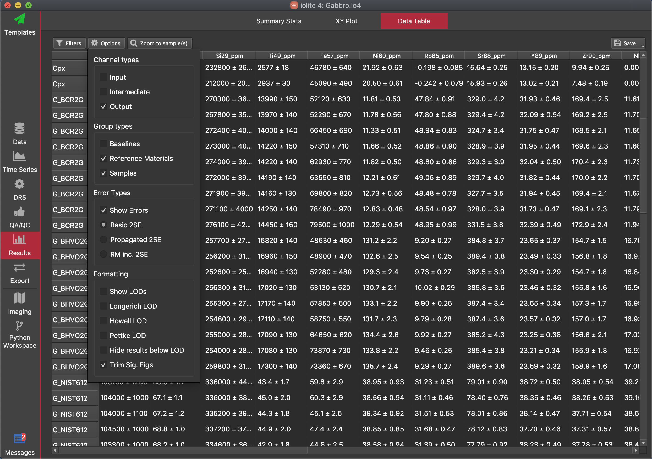
LODs can also be shown (for output channels only) by selecting the Show LODs checkbox. You can show the different LOD values (Longerich, Howell, Pettke) using the respective checkboxes. You can hide values below the calculated LOD by checking the "Hide results below LOD" option. This option uses the Pettke LOD value if calculated. If it has not been calculated, it uses the Howell value, and if that is not available, it uses the Longerich value.

The "Trim Sig Figs" option (on by default) trims the number of signficant figures shown for results according to their uncertainty. For example, if the mean of Sr88 for a selection is 288.343359 and the uncertainty (2SE) is 2.1, the value shown will be 288.3 (one additional significant figure beyond the uncertainty).

Filters Panel¶

The Filters Panel shows filters applied to the data table. You can add filters by clicking the button. Selecting certain options in the Options Panel automatically creates a filter, and those are shown in the Filters panel. You can also select an existing filter and remove it by clicking the button.

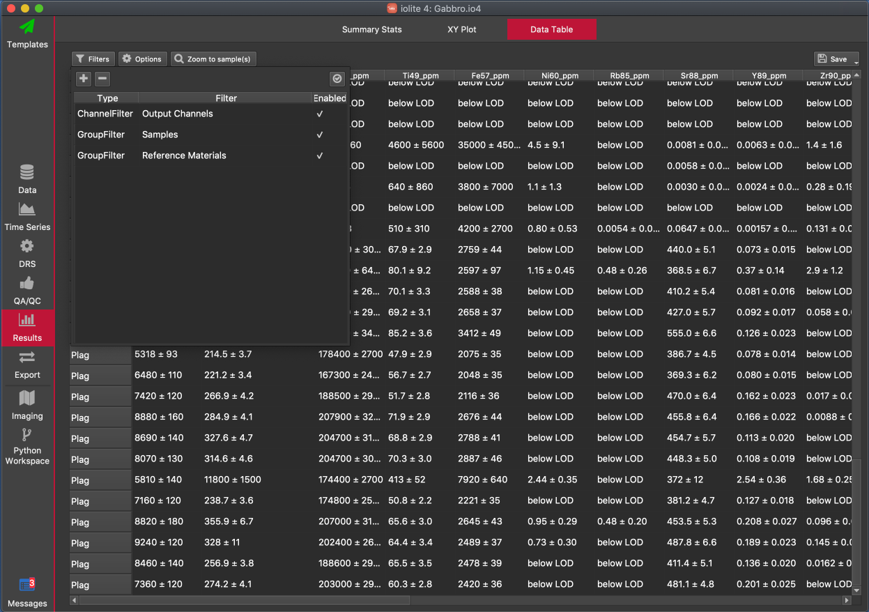
Filters that have been added are shown in a table in the panel. In the example above, there are three filters in the table. The first column of the table shows the type of filter, the second column shows the filter value, and the third column shows whether the filter is currently enabled or not.

Filters can be of the following types:

Group filter:

a filter applied to the name of the selection group (e.g. setting a group filter with a value of "G_BCR2G" will show only selections from the G_BCR2G group, if it is the only filter: see combining filters below).

Selection filter:

a filter applied to the name of the selection.

Channel filter:

a filter applied to the name of channels to determine if the column will be shown (e.g. setting a Channel filter of "Si" will show all channel with Si in their name, so Si29, Si29_CPS, Si29_CPS/Ca43_CPS and Si29_ppm will all be shown).

Result filter:

filter selections based on their result. For example, setting a Result filter of "Ti49_ppm > 2000" will show only selections with Ti49_ppm greater than 2000 ppm. See the note below about combining filters.

Metadata filter:

a filter based on metadata values. For example, you can filter based on spot size (height or width) using this type of filter.

Note

Datatable filters are combined in an OR combination. That is, any selection/channel/value will be shown if it matches any of the filter criteria. For example, if you have a Group filter "G_BCR2G" and another Group filter "G_NIST612", both BCR2G and NIST612 selection groups will be shown because the selections match either of the criteria.

You can enable/disable all filters at once using the button at the top right.

You can zoom to a particular selection in the Time Series View using the "Zoom to sample(s)" button.

You can save the values within the table by clicking the Save button at the top right, or by right clicking on the table and selecting the preferred export format (.csv or xslx file).

Tip

You can copy and paste values from the table into Excel (or similar) by selecting the data you want to copy and pressing Ctrl + c (Cmd + c on Mac) to copy the data to the clipboard. You can then paste the data into Excel etc. Use Ctrl + a (Cmd + a on Mac) to select all values within the table, then Ctrl + c to quickly copy the entire table.

Export View¶

The Export View allows you to export your results from iolite. You can choose to export your results to a file (either a comma-separated value .csv file or an Excel .xlsx file), or you can use a python script to export your results. When using a python script, there are very few limitations on how or where your results are exported. For example, you can export to a database using a database connection, or filter your results before export.

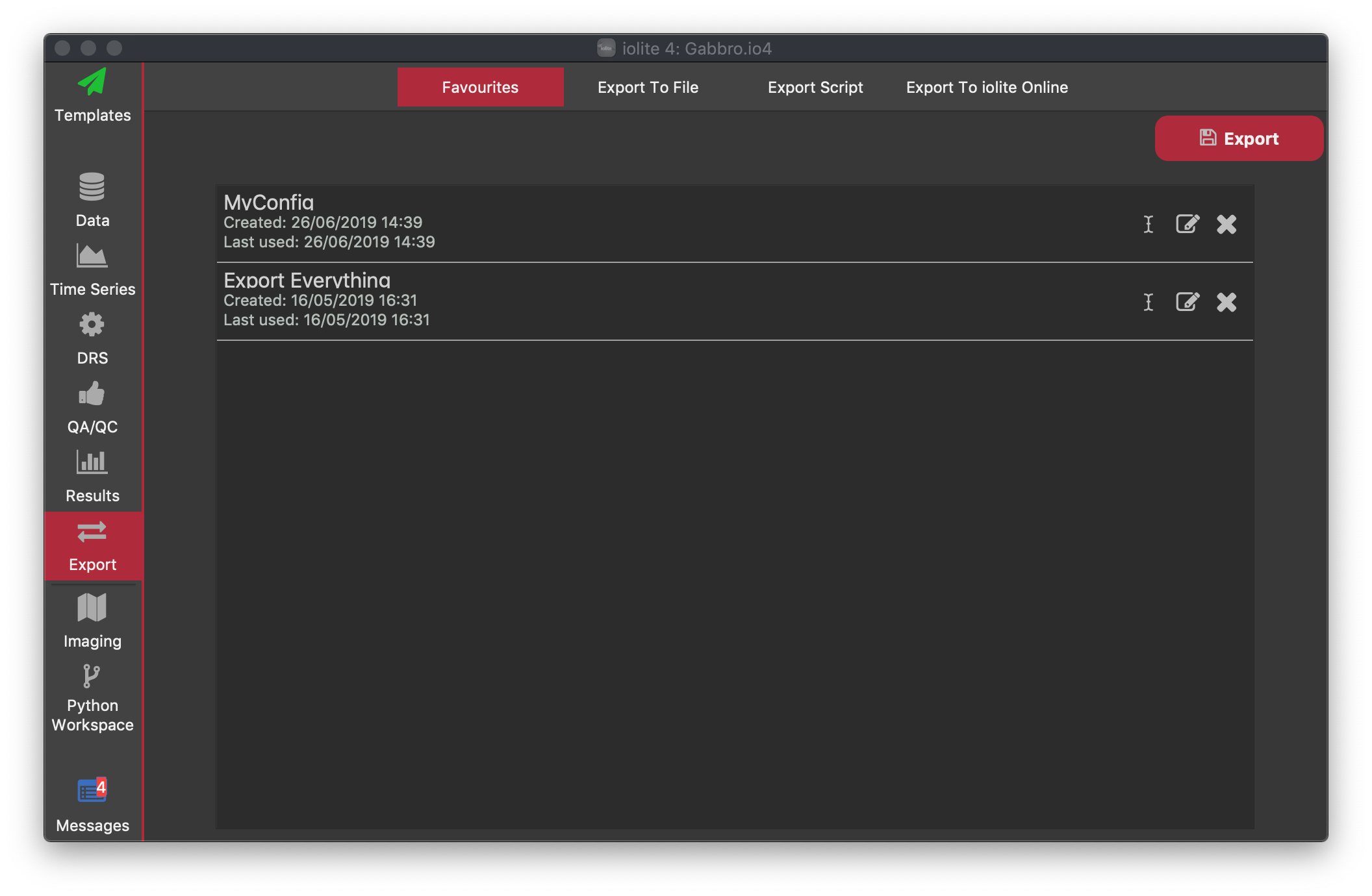
When exporting to file, once you have determined what you want to export (see Export to File below) you can save your settings to as a favourite configuration. These are shown in the Favourites tab, which will be empty until you have saved a configuration.

For each configuration, the name is listed along with the time and date it was created and last used. You can rename the configuration by clicking the icon. You can edit the configuration by clicking the icon. Clicking the icon will delete the configuration (this cannot be undone).

To use a favourite configuration, select it from the list and click the Export button in the top right. You will be prompted for the save file(s) location.

Export to File¶

The Export to File tab allows you to specify everything about the data you want to export. This includes the channels, selection groups, the file type and what statistics for each selection you want to report.

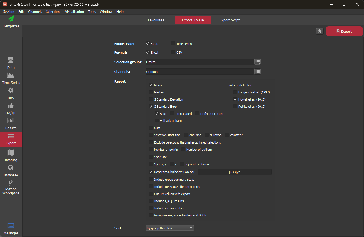
Export Type¶

Here you can select whether you want to export a single value (mean ± uncertainty) for each channel ("Stats"), or whether to export every value within each selection ("Time Series"). The Stats option is the most commonly used and the results are contained in a single file (see options below that may export additional files). The Time Series export will produce a separate worksheet (Excel export option) or separate text file (CSV export option) for each selection, which the value of each channel for each datapoint within the selection.

Format¶

Here you can select whether the output file is in Excel format (.xlsx) or comma-separated value format (.csv).

Selection Groups¶

Here you can select which selection groups you want to export data for. You can use the button to the right to quickly select groups. For example, if you wanted to export results for your unknowns (excluding your primary and secondary reference materials), you could select the "Samples" option. The groups to be exported are shown as a list, separated by semi-colons, with no spaces between names. You can delete any group you've added from this list by deleting the name from the list.

Channels¶

Here you can select which channels, or groups of channels, you want to export results for. The most common option is to export all Output channels by clicking the button to the right and selecting "Outputs". You can also add individual channels by selecting them from the Input, Intermediate and Output lists. The channels to be exported are shown as a list, separated by semi-colons, with no spaces between names. You can delete any group you've added from this list by deleting the name from the list.

Report¶

Here you can change what is reported for each selection. Typically for the "Stats" export type, you would export the mean and 2 standard errors, but it is also recommended to export the number of points and number of outliers. If including the standard errors (recommended), you can choose whether to export the basic 2SE (the 2SE of data points within the selection range, excluding any outliers), Propagated 2SE (the 2SE after error propagation) or the RMInc error (the propagated 2SE, with any uncertainty from the primary reference material added in quadrature). Any limits of detection (LODs) can be selected for inclusion in the export file.

You can replace values below the limits of detection with a default value (e.g. BelowLOD) by checking the "Report results below LOD as" option.

Tip

You can replace values below the LOD with negative LOD by typing -[LOD] into the "Report results below LOD as" field. For example, if your sample value was below the LOD value of 3.25, its value will be replace with -3.25.

You can also include any QAQC results by checking the "Include QAQC result" option. For Excel format exports, this will create a new sheet for each QAQC module. For .csv file exports, the table of results will be included in the main .csv file, and any plots will be saved as individual .png files.

Once you have set up your preferred export options, you can save it as a Favourite by clicking the button in the top right.

To complete the export process, click the red Export button in the top right. You will be prompted for the save file(s) location.

Export Script¶

You can use python scripts to create custom export procedures for iolite. These can either be stand alone python script (.py) files, or if you select the "Code" option from the dropdown menu, you can write your own script in the space provided.

To run the export script, click the red Export button in the top right. You will be prompted for the location you wish to export to, which may be ignored depending on your python instructions.

To save the export script location as a Favourite, or to save the contents of the code window as a Favourite, click the button at the top right.

Export to iolite Online¶

This functionality is coming in a new release soon. It will provide you with an online database to save your results and share them with others.

Imaging¶

The Imaging View contains all the features needed to create and inspect your images.

The view comprises four main tabs: Overview, Detail, Data Table, and Export. Additionally, while using the Overview and Detail tabs, there is a Setup tab and an Inspect tab.

Overview Tab¶

The Overview tab provides an view of all your images at once. Using this tab, you can set values for all images/channels and this is where you initially create your images using the Setup panel which you can show/hide using the Setup button, and should be visible by default. You can also import external images (that is, photomicrographs, SEM images, sample scans etc) in this tab.

When you first access the Imaging View, the main part of the window will show what pieces of information iolite needs to be able to create your images. Namely, these are a map type (CellSpace or From Selections), a selection group to plot, and a list of channels to create images for. Each of these parameters can be set using the Setup Panel (below) and once each of these pieces of information are provided, the checkbox beside the label will become ticked showing that iolite now has that piece of information.

You can show/hide the setup panel on the left hand side of the window by clicking the Setup button.

Overview Setup Panel¶

Using the Setup Panel, you can set the basic image paramters (image construction type, selection group to plot, channels to plot), as well as the shape and orientation, display parameters (colour table, filters), and import external images.

iolite cannot create any images without knowing the image type (CellSpace/From Selections), the selection group to plot, and the channels to plot. You can set these in the topmost section of the setup panel. If you have collected a laser log file (and imported into your current session), we recommend using the CellSpace option as this will plot the image in cell coordinates and show the true geometry. If you are unfamiliar with CellSpace images, we recommend reading the publication describing it in detail [5].

The Channels field shows a list of the channels to be used to create images. This is a semi-colon separated list of input, intermediate and/or output channels. Clicking the button to the right of this field shows a menu of channel names. You can use these instead of typing in the channel names. For example, clicking on the button, and selecting the 'Outputs' option will automatically add all output channels to the list of channels to be created. Alternatively, you can select individual channels from the Input, Intermediate or Output channel lists in the menu.

In the current version (v4.0.9), the cache option does not affect anything and can be ignored. This will be used in later versions to allow you to manage your computer's memory usage when working with large images.

If using the From Selections image construction, you can set whether the start, end, or center of each scan line is aligned using the Alignment option. If you select the Justify option, the starts and ends will be aligned and each scan line will be interpolated to have the same number of pixels.

You can also set the image width and height if using From Selections (for CellSpace images, this will be already completed using values from the laser log file). The Aspect Ratio will be shown and is the Width ÷ Height.

You can adjust the size and rotation of all images in the Overview tab using the Size and Rotation sliders. You can also mirror the images vertically or horizontally using the Mirror check boxes.

Once you have created images you can select which images values are adjusted when altering the gradient, scale bar settings etc (below) by clicking on the image in the main part of the Imaging Overview tab. This will place a check mark in a green circle in the top right of the image to show that it has been selected for adjustment. You can select all images using the Select All button, and deselect all images using the Deselect All button.

You can remove any channels from the Overview Tab by selecting them and clicking the button. If you remove a channel by accident and want to replace it, just select the channels from the dropdown list again. Images that are removed are not deleted, but rather are just not shown. Adding them back to the list of channels will replace them, along with any settings and filters you may have applied to them.

The Parameters section allows you to set the image gradient (also known as the the image color table); whether and where the scale bar is shown (i.e. the distance scale bar, not the color gradient scale bar), as well as the type of color scale. Options for the color scale are: Linear, Logarithmic, and ECDF (the 'empirical cumulative distribution function', see Rittner and Müller (2012)[#] for more details).

You can also set Lower and Upper color scale limits here. Setting the lower limit means that any pixel value equal to or lower than this value will be set to the first color in the color gradient. Similarly, setting the upper value means that any value equal to or greater than this value will be set to the last color in the color gradient. If your image data has outliers, it may reduce the number of colors used to represent your images to a small part of the chosen color gradient. Setting manualy Lower and Upper limits can help this, or you can try using the 'TwoSDofMean' or 'TwoSDofMedian' options that will automatically set the lower limit to the mean/median - two sd of your pixel values.

In general, using the ECDF will maximise contrast for your images, but will normally result in a non-linear color scale making it more difficult to conceptually match a color to a concentration value. You can, however, use image interrogators to determine concentrations for Regions of Interest (ROIs) if a more definitive value is required for a particular area.

To add a filter to an image(s), select the image(s) in the main part of the Overview Tab. In the Filters section of the Overview Setup Panel, click the Add button. This will show a list of available filters. At the time of writing, these include the following:

Box2D: Applies an n x m box filter to both the rows and columns of the image. You can adjust the number of rows and columns.
Box columns: Same as for Box2D but only applied to image columns
Box rows: Same as for Box2D but only applied to image rows
Expand by Interpolating: expands the image to have the same number of rows/columns. This can be useful if additional resolution in either the x or y direction is required.
Gauss2D: Applies an n x m 2D gaussian filter to the image.

By default, Box2D and Gauss filters are 3 x 3 kernels, Box column filters are 1 x 3 filters, and Box row filters are 3 x 1 filter. The size of box and gauss filters can be adjusted by selecting the filter in the list and clicking the Setup button. The maximum filter size is 24 rows/cols.

Python Workspace¶

The Python Workspace View provides a workspace for interacting with iolite and your data using Python.

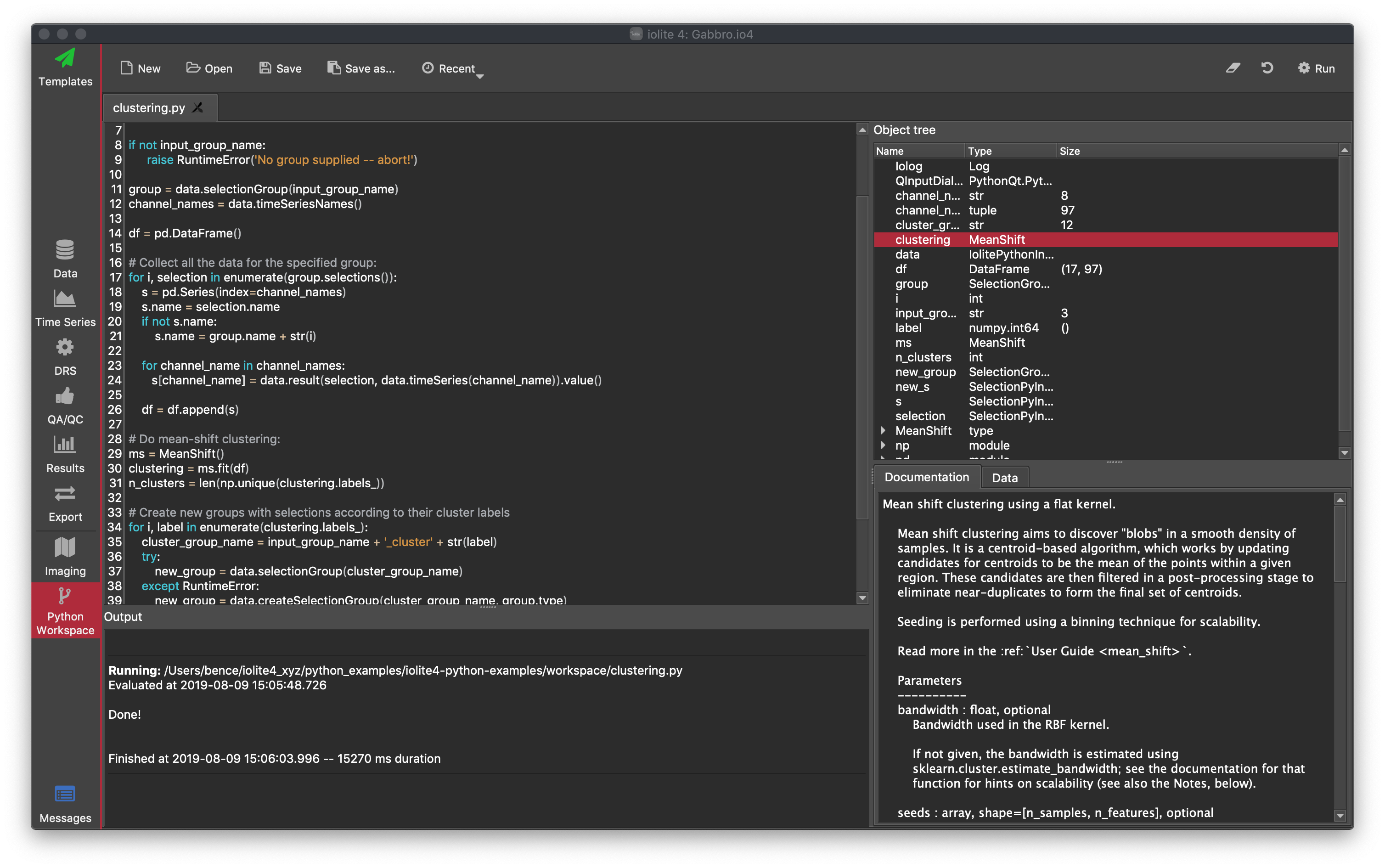
Along the top of the workspace is a button bar, where you can open, save and run scripts. Clicking the Run button will run the currently displayed script. You can also reset the workspace using the button. Clicking the button will clear the output panel (see below).

The main panel on the top left is an area to write python scripts. You can also load existing scripts using the Open button in the button bar along the top of the Workspace. You can have multiple scripts open in this panel (each will be shown as a tab). Only the currently displayed script is executed when you click the Run button in the button bar. Beneath this script area is the output panel. This panel shows the console output from running your script

Messages View¶

The Messages View shows you a log of all messages generated by iolite. This includes messages telling you what effect your action have had (e.g. if you have added selections using criteria, the number of selections created will be logged in the Messages View), and if any errors have occurred.

There are four categories for messages:

Information:: provided to log what has happened during the normal course of processing your data.
Warning:: a message to let you know something has happened that not have been expected, but may not necessarily be an error.
Error:: a message to let you know an error has occurred.
Debug:: these messages provide information about the state of iolite at certain times to help diagnose errors.

There are four icons in the top left that show/hide each of the four categories. By default, debug messages are hidden.

You can clear all messages in the log by clicking the Clear button in the top right, and save the log (as a .json file) by clicking the Save button in the top right.

Tip

You can search for messages using the Search... field at the top of the table of messages.

Keyboard Shortcuts¶

(NOTE: Scroll table to the right to see additional notes)

Grouping	Function	Windows	Mac	Notes
Sessions	New Session	Ctrl + n	Cmd + n
	Save Session	Ctrl + s	Cmd + s
	Save Session As	Ctrl + Shift + s	Cmd + Shift+ s
	Open Session	Ctrl + o	Cmd + o
Window controls	New iolite Window	Ctrl + =	Cmd + =
	Show Processing Templates View	Ctrl + 1	Cmd + 1
	Show Data Browser View	Ctrl + 2	Cmd + 2
	Show Time Series View	Ctrl + 3	Cmd + 3
	Show DRS View	Ctrl + 4	Cmd + 4
	Show QAQC View	Ctrl + 5	Cmd + 5
	Show Results View	Ctrl + 6	Cmd + 6
	Show Export View	Ctrl + 7	Cmd + 7
	Show Messages View	Ctrl + 8	Cmd + 8
	Show Notes Panel	Ctrl + '	Cmd + '
	Show Help Panel	F1	F1
	Open Preferences	Ctrl + ,	Cmd + '
Data Browser View	Import Mass Spec Data	Ctrl + i	Cmd + i
	Import Laser Log File	Ctrl + Shift + i	Cmd + Shift + i
	Copy sample info (Sample Browser)	Ctrl + c	Cmd + c	Copies sample info to clipboard
Time Series View	Create new selection	Hold Ctrl + left click and drag	Hold Cmd + left click and drag
	Enter Edit mode for selection	Hold Shift + left click	Hold Shift + left click	Click on a selection
	Show selection details	a	a	Selection must be in edit mode
	Delete a selection	Delete/Backspace	Delete/Backspace	Selection must be in edit mode
	Delete All Selections in Group	Shift + Delete	Shift + Delete	A selection must be in edit mode
DRS View	Clear IS values in Trace Elements	Delete	Delete	One or more rows must be selected
	Copy IS values from table	Ctrl + c	Cmd + c
	Paste IS values into table	Ctrl + v	Cmd + v
Proc Template View	Delete current action(s)	Delete	Delete

Notes Panel¶

You can record notes as you are processing your data in the Notes Panel. To show the panel, go to the Window menu -> Notes, or press Ctrl + ' (Cmd + ' on Mac). This will show the Notes panel, which can be resized to suit, or be dragged to a new docking location at the top, left, right or bottom of the main iolite window by clicking and dragging the title bar of the panel. A red rectangle will appear when you drop the panel to one of the docking locations. You can also drag the panel out of the window to create a floating panel that is always over the top of the main window so that you can see it and add notes to it.

Notes are saved within your session file, so they remain as a record even after closing and re-opening a session. They are a good way of recording data processing decisions and the effects of certain choices. They can also be a good place to store observations for later review. Closing the Notes Panel by clicking the close button does not destroy the notes contained within the Panel. It simply hides the panel until needed again.

You can format text in the Notes using the Markdown syntax. There are a lot of guides to this very simple text formating scheme on the internet, but briefly, you can mark text as bold by enclosing it with two asterix (e.g. **this text** will be shown as this text). You can mark headings with hashes. For example #My Heading will be shown as a major (level 1) heading. ##My 2nd Heading will be shown as a secondary (level 2) heading, and so on. If you need to use any of the formatting symbols (e.g. #) without the formatting, you can prefix the symbol with a backslash.

You can also drag any plot into the Notes Panel by holding the alt key and dragging the plot into the Notes Panel. As soon as you start dragging the plot, a small thumbnail of the image will be under the mouse cursor.

Note

QAQC plots can be copied and pasted into the Notes. Right click on the plot and select Copy and then paste into the Notes using Ctrl + v (Cmd + v on Mac).

Any images included in the Notes Panel are static, so they do not update if you change the settings etc. This can be a good way of recording the effect of certain settings.

You can save your notes as a html file by right clicking on the Notes and selecting Export.