U-Pb Geochronology

This is a step-by-step guide to reducing simple U-Pb data using iolite v4. You should have already installed iolite v4 before beginning this tutorial.

To follow along, you can download the examples files here.

The example files include:

Zircon.csv:

An Agilent mass spectrometer data file, format dd MM yyyy h mm ss.

Zircon_log.csv:

A laser log file, describing the name of each ablation spot, when it started and ended and its x,y location (although the x and y coordinates are not used in this example)

This data set includes analyses of reference materials 91500, Plesovice and Temora and an unknown called DRO4 acquired as 30 second, 5 Hz, 18 μm diameter spots. Most spots have ~ 15 seconds between them and include cleaning pulses. Occasionally, longer delays were used between spots to help define the background.

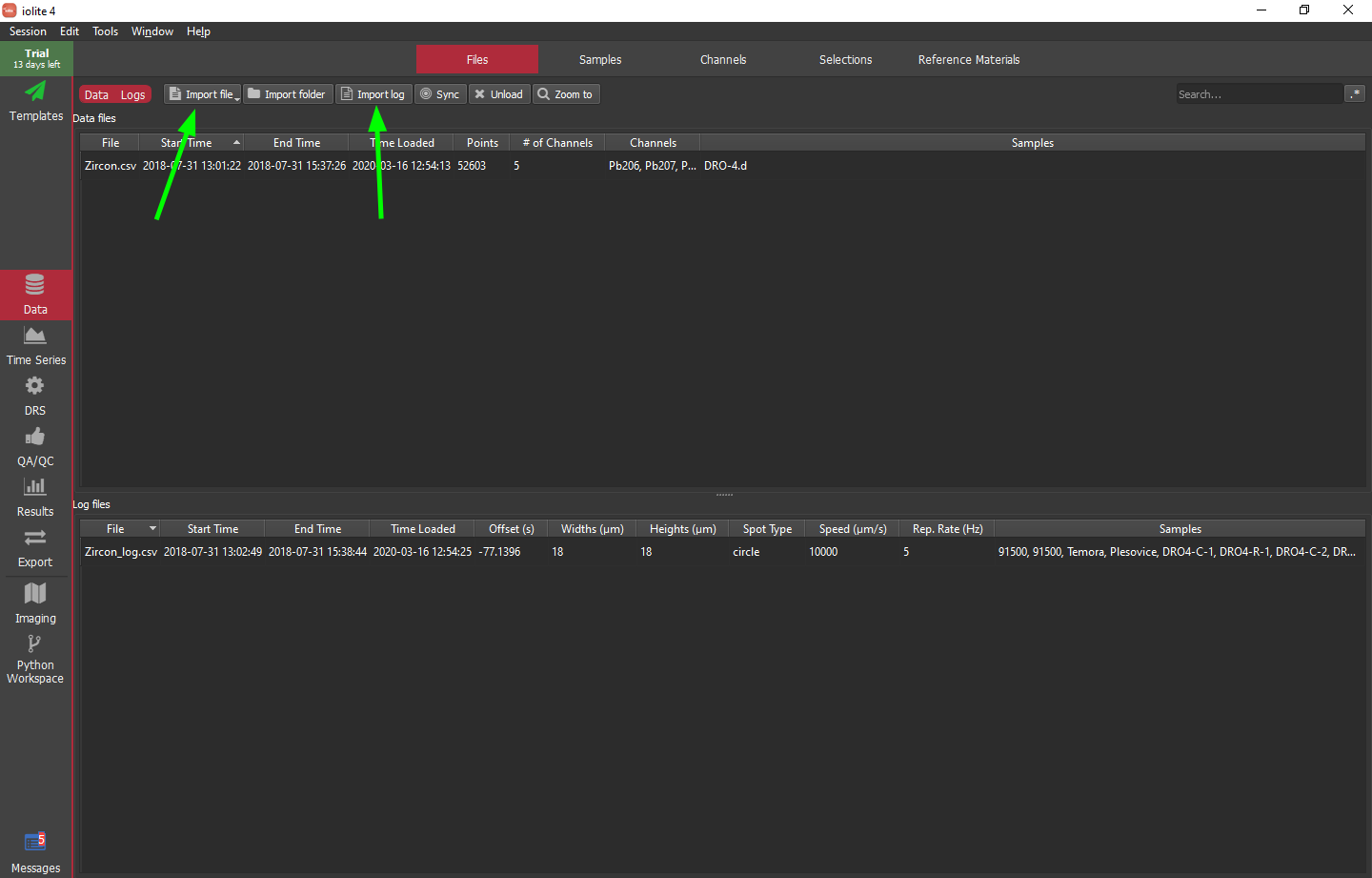
To import the data and log files, click the "Import file" and "Import log" buttons, respectively, as indicated by a green arrows in the image below.

Hint

If nothing shows up in the data files list after trying to import Zircon.csv, most likely the Agilent date format specified in the preferences does not match the contents of this file. You can check iolite's messages (button in the bottom left of the main window) to see the date format of the file and use this information to set the date format in iolite's preferences.

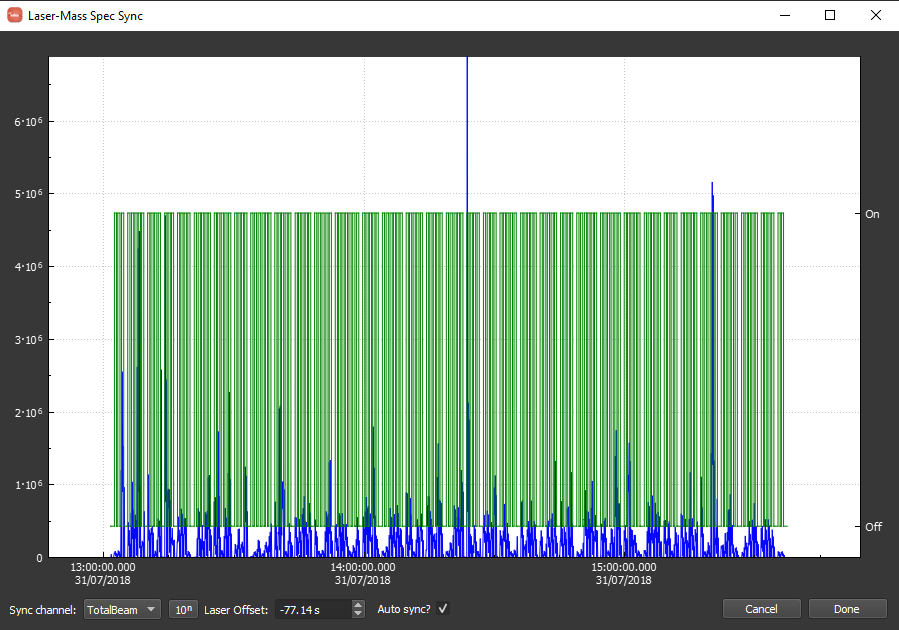
When synchronizing the log file, it should look as below. Note that the time offset between the data and log is approximately -77 seconds. You can (should) zoom in to verify that the automatic synchronization was successful. If it was not, unselect "Auto Sync?" and manually adjust the offset. Note that you can zoom in by scrolling and pan by clicking and dragging. You can adjust the offset graphically by shift-clicking and dragging. Also, as you zoom in, the labels specified in the log will begin to appear as there is enough room. When you are happy with the syncing, you can should click "Done" in the bottom right.

The hard way

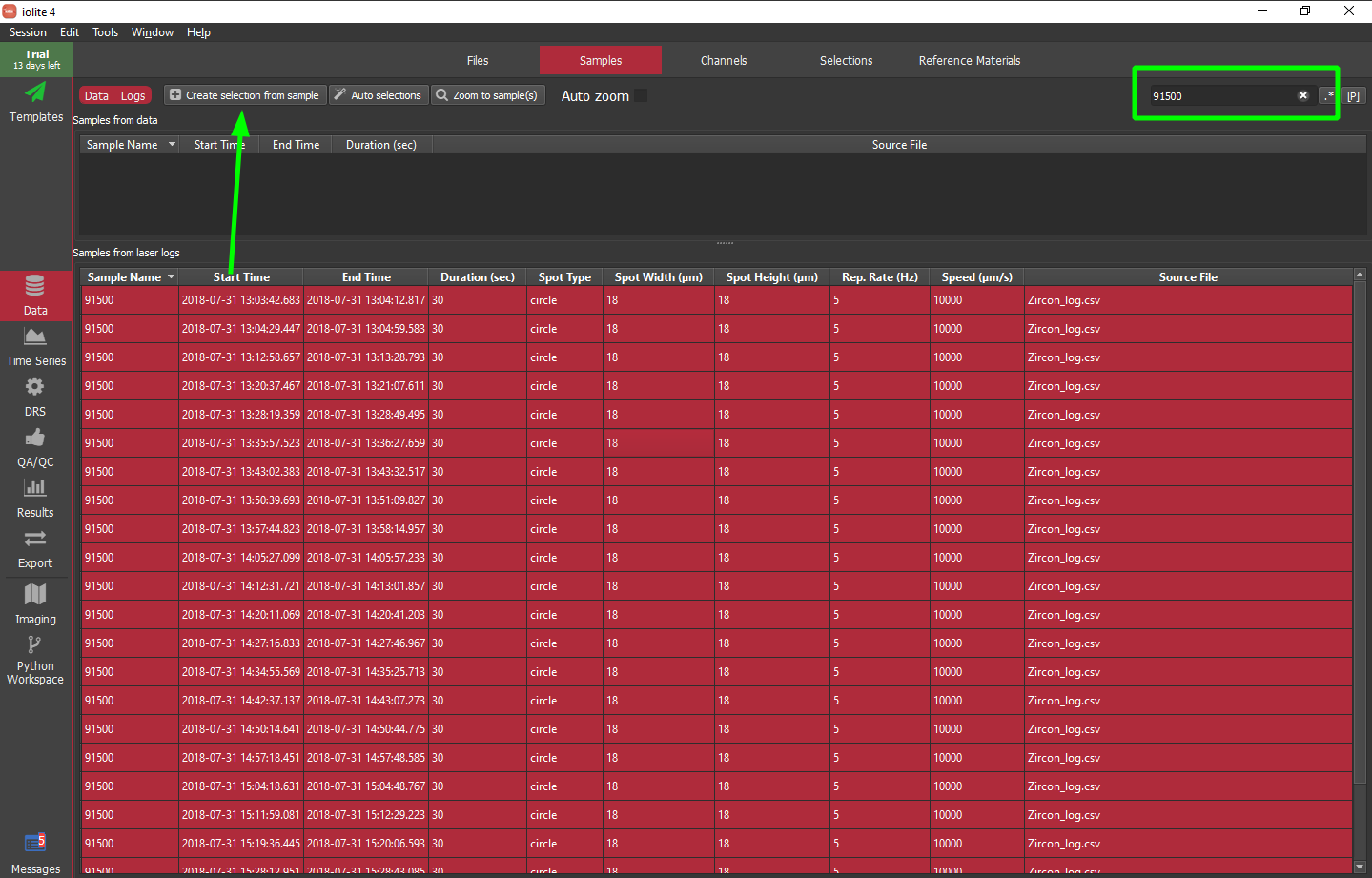
iolite has long supported the use of laser logs to define selections based on labels provided when setting up your analyses in your laser ablation software. In iolite 4 this is easier than ever -- select the laser log samples you want to create selections for then click the "Create selections from sample" button highlighted with a green arrow below. Alternatively, you can search the labels using the field in the upper right. This way you can find all of the samples matching some label, e.g. 91500, then select all of those samples and add them to the Z_91500 selection group.

Note that there is also the really hard way of setting up selections manually. We will not cover that approach here as it is very tedious, but it is possible. To learn more about making selection groups and selections manually, see this section.

The easy way

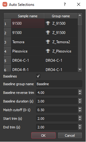
The so-called hard way above is not actually that difficult, but can be a bit repetitive when you have many groups to create. iolite 4 comes with a handy feature called "Auto selections" that uses a string matching algorithm to match sample labels to reference materials and other selection group names.

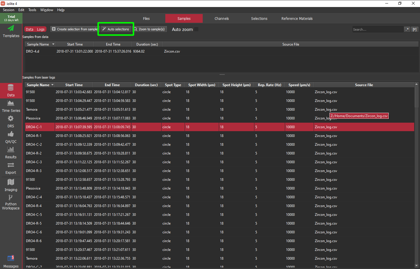
When you click the "Auto selections" button you will see a dialog as below. The table shows you how it is mapping sample names to groups and indicates a if that is a reference material. Note that this works best if you label your samples similar to the reference materials defined in iolite. The "match cutoff" parameter can be adjusted if things are not mapping as expected where 1 = perfect match and 0 = completely different. You can also use the sample metadata to define baseline selections automatically. In this example, I have found that using a reverse trim of 4 seconds and duration of 3 seconds works pretty well.

Note

The algorithm maps DRO4-C-1 to a new group called DRO4-C-1 and the remaining DRO4 labels are close enough to that that they will also assign to the DRO4-C-1 group.

The baseline selections created using "Auto selections" above might not be ideal in this particular case as the experiment was designed with longer delays for gas blank periodically but not between every analysis. Perhaps a better way to setup baselines for this experiment would be to use Tools ‣ Automatic Selections ‣ From Channels.

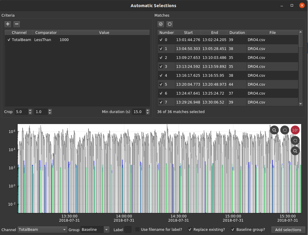
For this dataset, I added a single criterion: TotalBeam < 1000, then I cropped the beginning and end by 5 and 1 seconds, respectively. Importantly, I specified a minimum duration of 15 seconds so that it only matches the larger gaps in the data. The group name ("Baseline") should be specified on the bottom of the window and "Baseline group?" should be selected. Finally, click "Add selections" in the bottom right.

Hint

If you are adding selections to a group that already contains selections be sure to toggle (or not) the "Replace existing?" option. If you aren't careful, you can end up with selections that are on top of each other which can cause problems.

Running the DRS

The U-Pb data reduction scheme (DRS), like other DRS can be accessed from the "DRS" tab on the left side of the main window. The main feature that sets the U-Pb DRS apart from others is its down-hole fractionation correction. In order to do this correction we must have a proxy for ablation depth, the most logical of which is time. Therefore, a critical step in the U-Pb DRS is figuring out the "beam seconds" channel.

For this experiment, the settings as shown below work fine. We will use Z_91500 as our reference material, use an exponential fit by default and use the laser log for the beam seconds and mask.

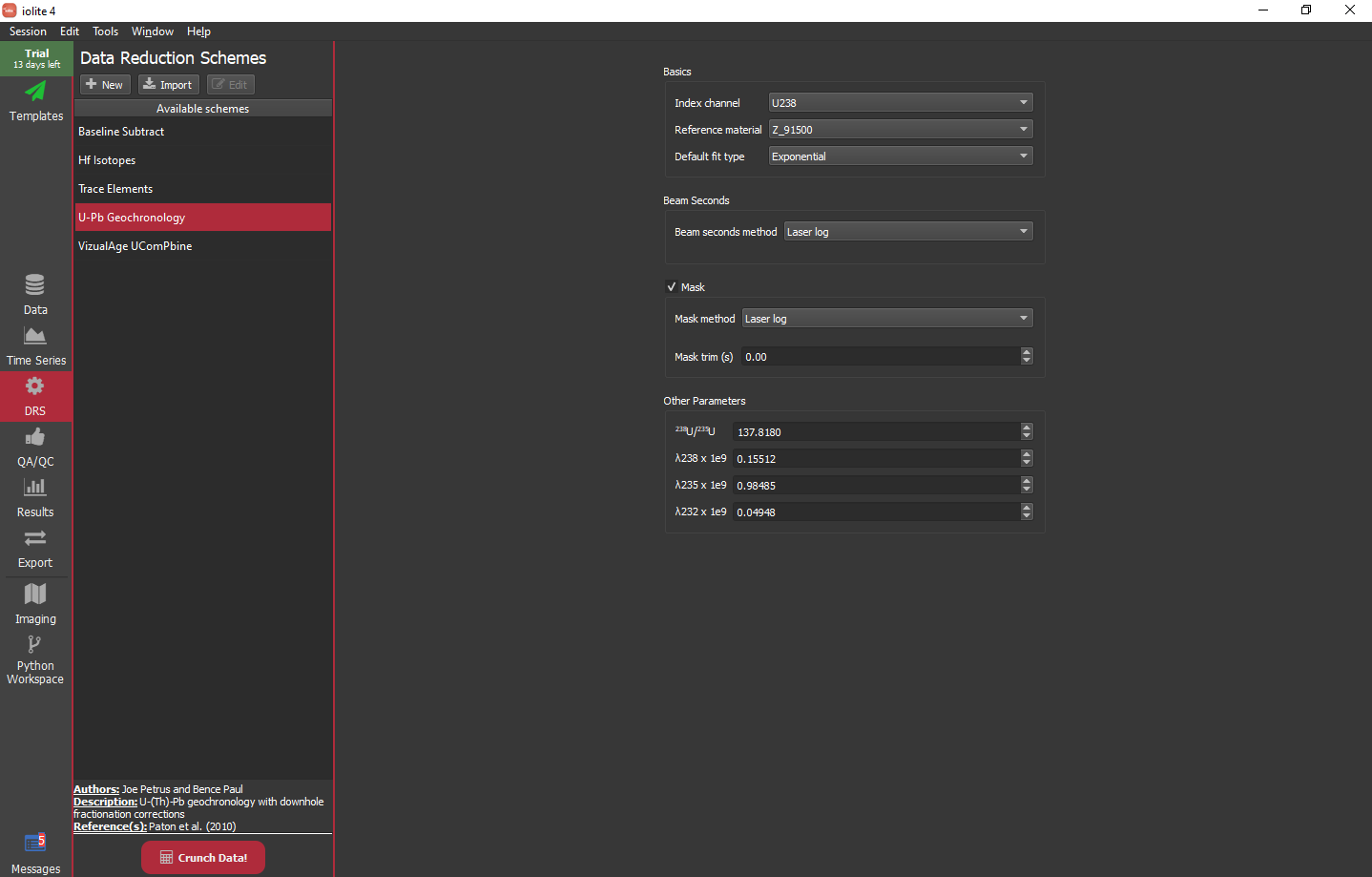
The settings available for the U-Pb DRS are as follows:

Index channel:

All of the channels calculated by this DRS will be referenced to the time of the channel specified here. This only really makes a difference if you have input data with differing time arrays.

Reference material:

The external reference material used to calibrate the final channels.

Default fit type:

The function used to model down-hole fractionation by default (it can be changed later).

Beam seconds method:

The method used to determine beam seconds: jump threshold, cutoff threshold, gaps between samples, or laser log (preferred).

Beam seconds sensitivity:

Sets the jump or cutoff threshold (only available for certain methods).

Beam seconds maximum:

Sets the maximum for beam seconds, e.g. if you know your spots are never longer than 60 seconds, you can specify that to help guide the calculation (only available for certain methods).

Mask:

Check to indicate whether to mask the calculated channels. Masking helps to clean up the calculated channels visually as ratios usually tend to be erratic during backgrounds which make it hard to see what is happening during ablation without carefully zooming in on the data. Masking does not normally affect results unless your masking is not setup properly and/or your selections overlap masked data.

Mask method:

The method used for masking: cutoff (based on index channel) or laser log (preferred).

Mask trim:

This adjusts the mask's on/off times by the amount specified.

Other parameters:

Isotope ratios and decay constants. Only adjust these if you are sure you know what you are doing!

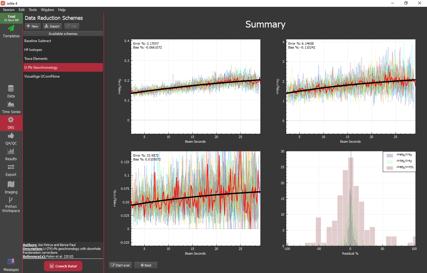
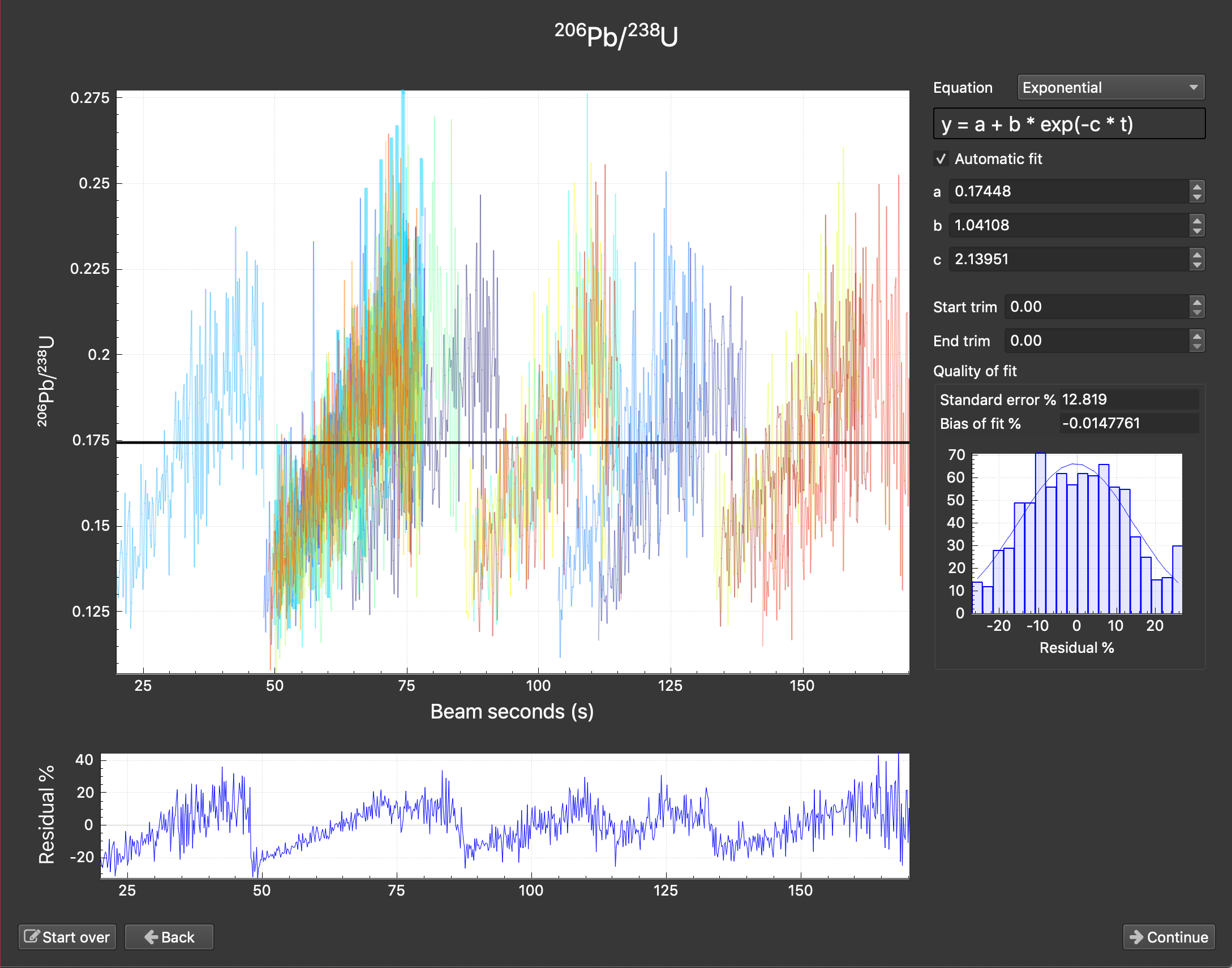
With the DRS configured, you can click the big red "Crunch Data!" button at the bottom of the DRS list. If everything has gone according to plan, you will be presented with the first down-hole curve fit window for ²⁰⁶Pb/²³⁸U:

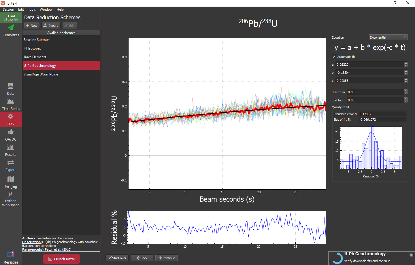
The main plot here shows the reference material plotted as ratio vs beam seconds. It includes the individual analyses (lighter line weight, varying colors), the mean of those analyses (heavier line weight, red) and the current fit to the mean (heavier weight, black). The lower plot shows the residual of the fit vs the mean and the small plot on the right shows the distribution of that residual. If you are happy with the fit, you can simply click the "Continue" button on the bottom. If you want to change the fit type, specify function parameters manually (rather than automatically), or trim the data the fit is applied to (e.g. if you have a wonky beginning and/or ending) you can do so with the controls in the upper right of the window. Once you click continue, you will be presented with the same sort of view but for ²⁰⁷Pb/²³⁵U and ²⁰⁸Pb/²³²Th.

When you are finished you will see a summary as shown below.

Hint

You can alt + click and drag the various plots to drop them into the notes or another program (e.g. image editor). Alternatively, you can right click and select save or copy.

Using QA/QC modules

iolite 4 includes concordia and discordia age QA/QC modules to help you ensure data quality. In this example, we have analyses of Plesovice and Temora that we can check. The QA/QC modules can be accessed much like the DRS modules -- by selecting the QA/QC tab on the left side of the window and then the desired module from the list. To setup the module, click the "Settings" button. For the concordia age module we can indicate which group to check (Plesovice below) and how close it must be to the accepted value (if it is a reference material with "Age" data) in order to pass.

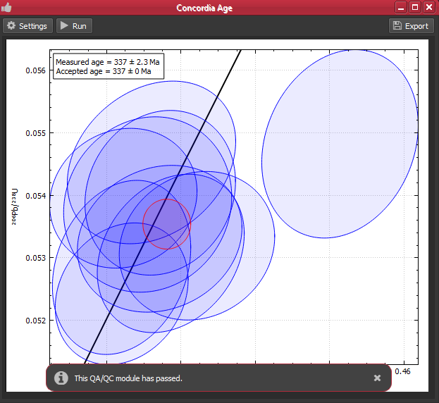
Hint

If you are routinely analyzing the same reference materials with the same conditions, you can probably make use of processing templates to automate this entire process, including a QA/QC check.

Hint

Setting an acceptable percent difference is most useful when used in conjunction with processing templates. In this case, if the QA/QC modules pass the template will proceed and export results, if not it will halt and you can investigate.

Making adjustments

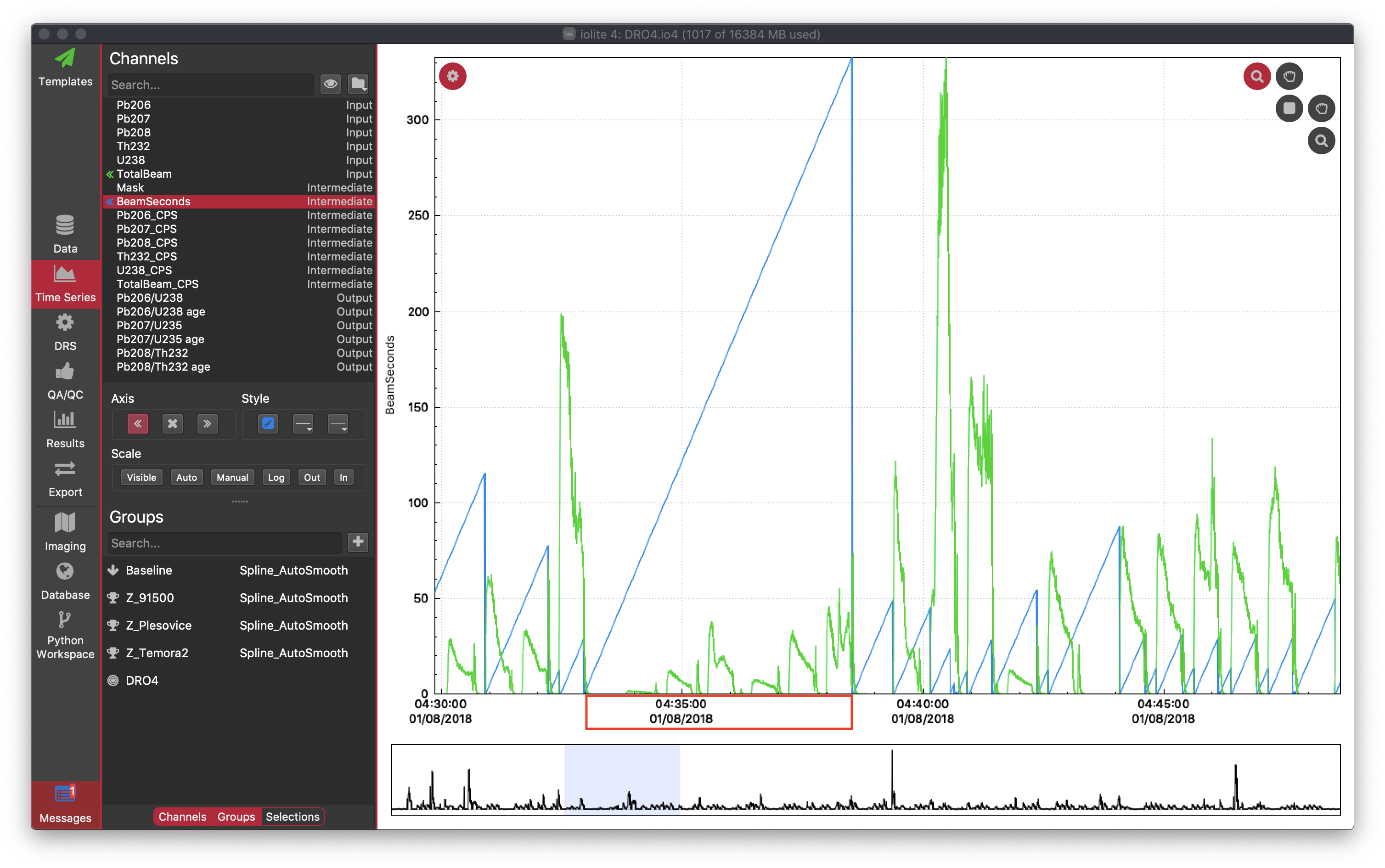
As the laser ablates through minerals it is fairly common to encounter parts of the target that are either compromised (e.g. by common Pb or Pb loss) and/or contain different domains and/or ablate through the target. Due to the high precision demands of geochronology, it is a good idea to inspect the various signals coming from each spot to be sure what you have selected to represent that spot is indeed the best representation. Below you can see a time series view

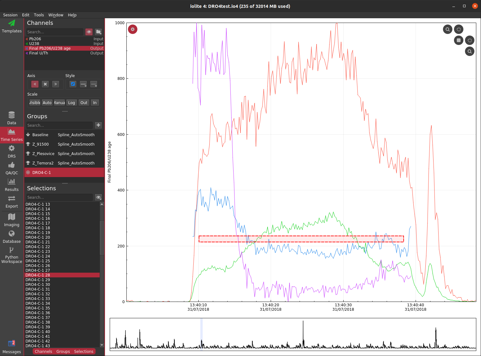
Although this can be very insightful, it can still be tricky to figure out which (if any) part of this analysis is "good". There is clearly a big difference between the first ~ 5 seconds and the remainder in terms of age and U/Th ratio, so it probably does not make sense to treat the whole thing as one analysis. We could split it into two selections based on the U/Th and 206/238 age, but it is hard to tell if these are concordant or discordant, and if discordant, whether it is due to common Pb or Pb loss.

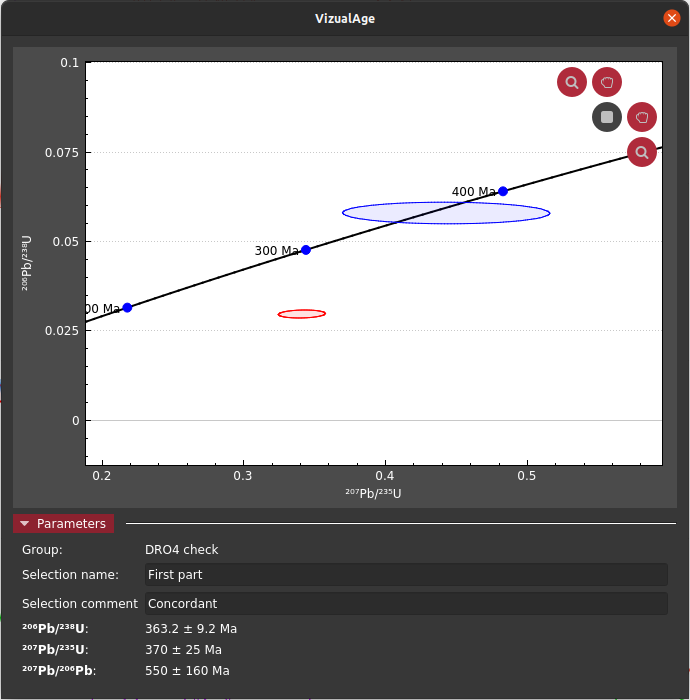
To simplify this process, VizualAge (original paper) was created. This allows you to see how a selection plots in concordia space as you adjust it in realtime versus the other selections in its group. For this particular selection, we can see that the first part is concordant and the latter part is discordant most likely from modern Pb loss.

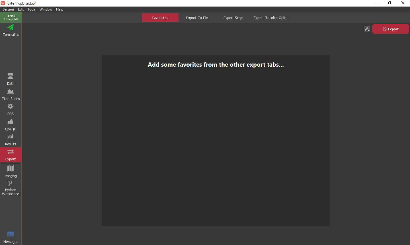
Exporting results

To export the data for subsequent use in, e.g. IsoPlot, we can go to the "Export" tab on the left side of the main window. By default this will show you a list of your favorites which may be empty when you are just starting out.

For this experiment, we can go to the "Export To File" tab along the top and set it up as shown below. Notably, we want to make sure we export "propagated" errors when available.

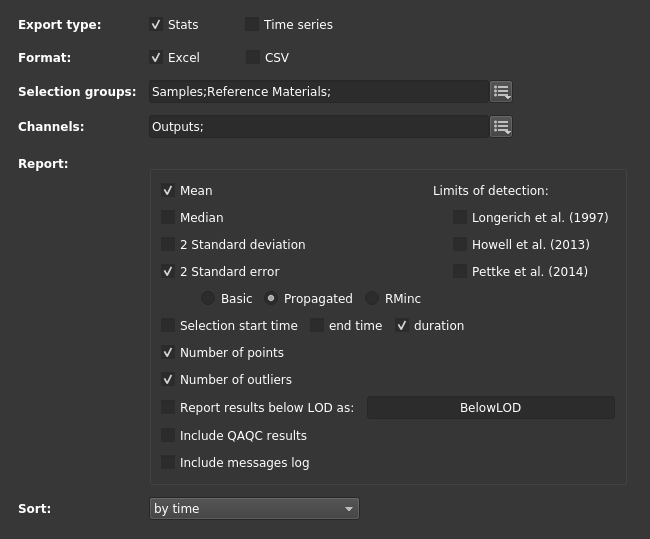
Once we are happy with the settings we can (optionally) save those as a favorite by clicking the star button in the upper right and then click the "Export" button also in the upper right. This process finishes relatively quick and a popup message is shown along the bottom of the window providing easy access to open the export folder or file.

Problems you may encounter

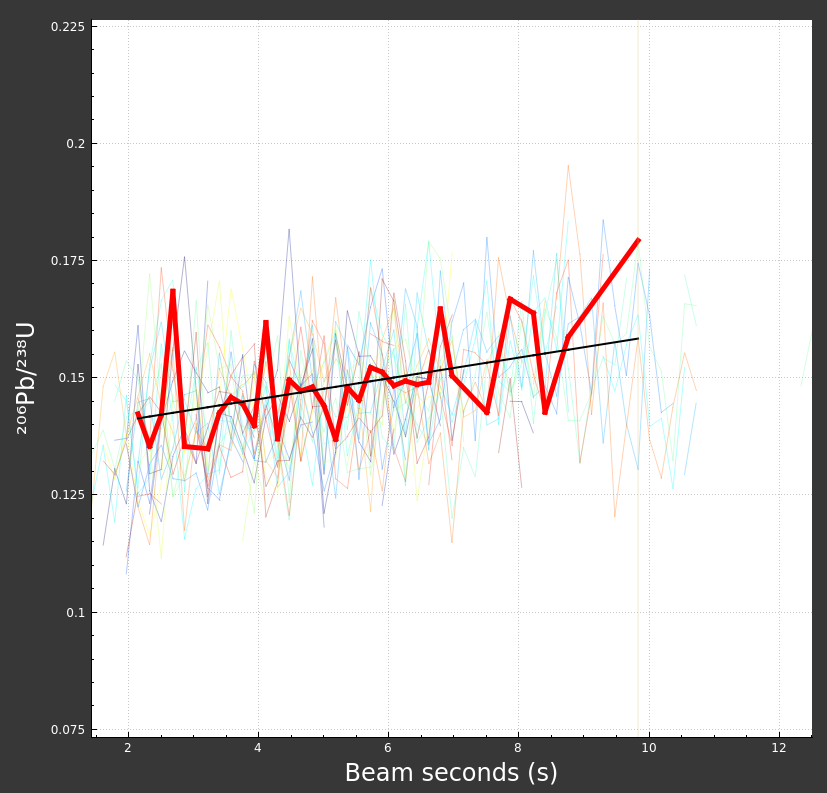
1. Bad beam seconds: If you are creating the beam seconds channel based on a cutoff or jump rather than using file or log metadata, it may take some guess work to determine a suitable value. A tell-tale sign that something is wrong with your beam seconds would be a down-hole fit window that looks as below.

If you were to look at the "BeamSeconds" channel in the time series view you would see that channel continue to rise over multiple spots as below.

To remedy this, try using a different index channel and/or cutoff/jump threshold. Better yet, use a laser log.

2. Bad mask: Similar to above, if you are not using laser log meta data for masking, it is possible to mask part or all of your reference material data. If you were to do that, it might look as below:

Or if you have masked all the data, you might even see something that looks like this:

If that is the case, you can safely "ignore" the warning and try different settings.

3. Poor down-hole fit: Depending on the nature of your data and the default fit type, getting a good down-hole fit may require some tweaking. For the example data set used here, the defaults do a pretty good job. However, if we were to adjust the start and end crop you can see that the resulting fit is not good:

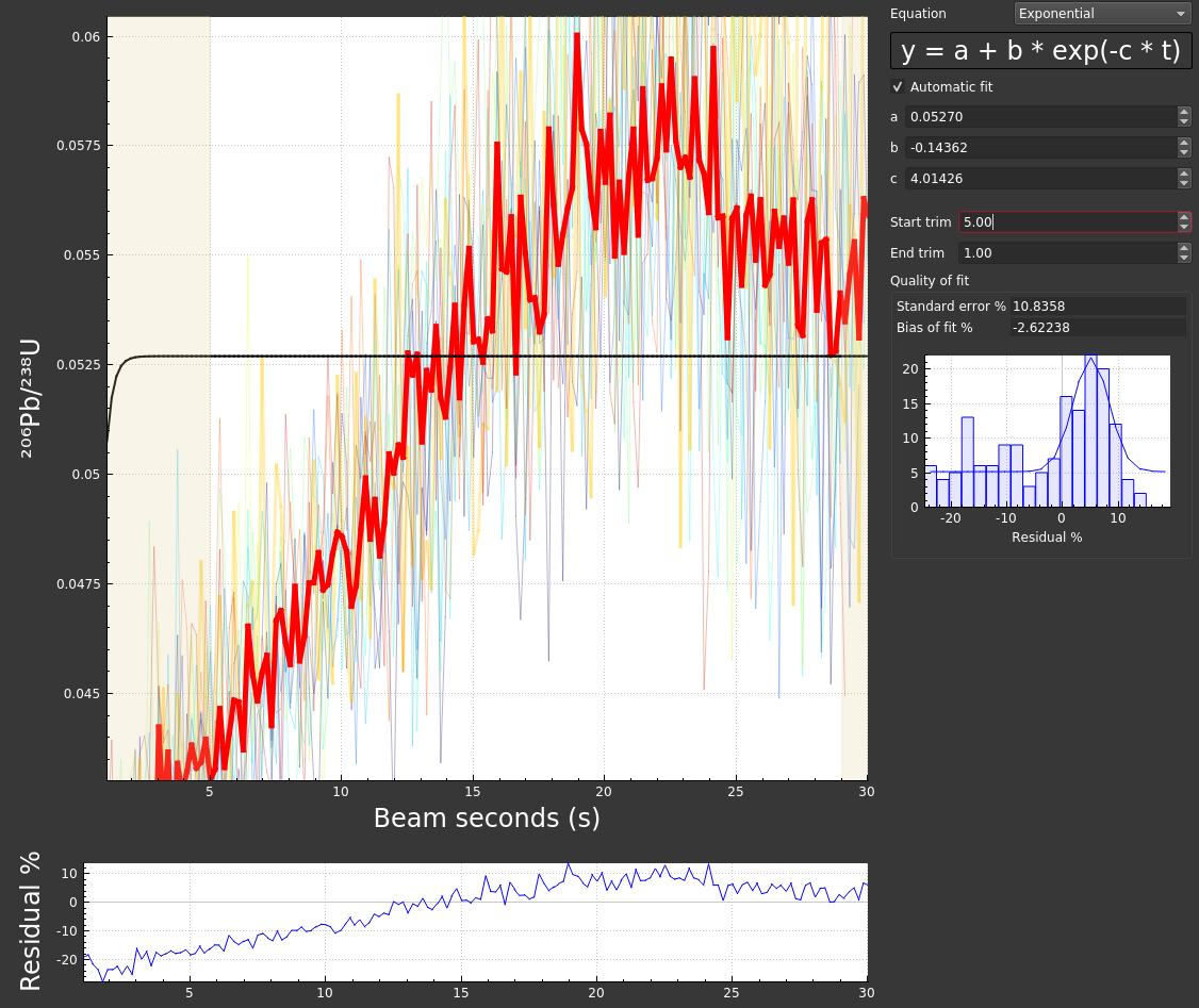
If the fit (black line) does not seem to do a good job modelling the down-hole trend (red line), you can adjust the fit type, trims, and/or uncheck "automatic fit" and try adjusting the equation parameters manually (usually this is not necessary).