Trace Elements

Here is a step-by-step guide to reducing trace element data using iolite v4. You should have already installed iolite v4 before beginning this tutorial.

Note

Please note that in this tutorial, every task will be done in long-form. That is to say, we won't be using any of iolite's shortcuts or automated tools in this tutorial. This is so that you are aware of what these tools do automatically, and so that you have a better understanding of the entire process. Also, please note that there are many ways to process your data in iolite. What is presented in this tutorial is just one workflow that helps beginners understand the basics of iolite a little better.

Note

If you have any questions or comments about this tutorial, please see the dedicated forum post here

This example is from a session where several minerals in a gabbro sample were measured. It's a good example because several different phases (minerals) were measured and a couple of different secondary reference materials were analysed (as they should always be). The secondary standards are basalt glass standards BCR-2G and BHVO-2G. The different minerals measured include some titanomagnetite (labelled as "Opaq_x" in the log file), plagioclase (labelled as "Plag_x" in the log file), olivine (labelled as "Oliv_x" in the log file), and clinopyroxene (labelled as "Cpx_x" in the log file). You don't need to know what these minerals are for this example to make sense. You just need to know that they have different elemental concentrations and

Hint

Adding multiple secondary reference materials is always a good idea. They give you the best estimate of your analytical performance, and only take a few minutes extra to measure.

You can download the example files from this link.

The example dataset includes three files:

Gabbro_data.csv:

An Agilent mass spectrometer data file.

Gabbro_log.csv:

A laser log file, describing the name of each ablation spot, when it started and ended and its x,y location (although the x and y coordinates are not used in this example)

Gabbro_IS_values.txt:

A tab-delimited text file with the internal standard concentrations for each spot.

Once you have unzipped the example file somewhere you can find again, we can start iolite. We'll begin a new session by clicking on the New button on the far left.

This will open the main iolite window.

If this is the first time you've used iolite, it's a good idea to have a look around. You can refer to the User Interface Guide for more information about each part of iolite. One of the key parts of the interface is the tab bar running along the left hand side of the window. Here you can see the major parts of the iolite interface which correspond to the major tasks in your data reduction (e.g. viewing results, performing QAQC, exporting your data etc). We'll start off in the Data Browser (labelled 'Data'). This has several tabs along the top: Files, Samples, Channels, Selections and Reference Materials. By default, you start in the Files Browser where we import files and can view information about the files that have been loaded.

To begin with, we are going to import the mass spec data. This is an Agilent file, so it doesn't have a standard timestamp format. We have to specify that in iolite's Preferences. If you are importing data from any other mass spec apart from Agilent and X-Series II instruments, you can skip this step as the other files have set timestamp formats. Preferences are accessed by going to the Session menu on Windows, or the iolite4 menu on Mac, and selecting Preferences. In the Import section, you can set the timestamp format for Agilent and X-Series II files. For this example, we need the format dd MM yyyy hh mm ss. This is the first option in the list, so we'll select that and click the Save button at the bottom of the window.

Tip

The time format box is editable. That is, you can type your own format into the box. There are a list of suggestions based on common formats, but if your format is not one of them, you can just type it in, or edit one of the suggestions.

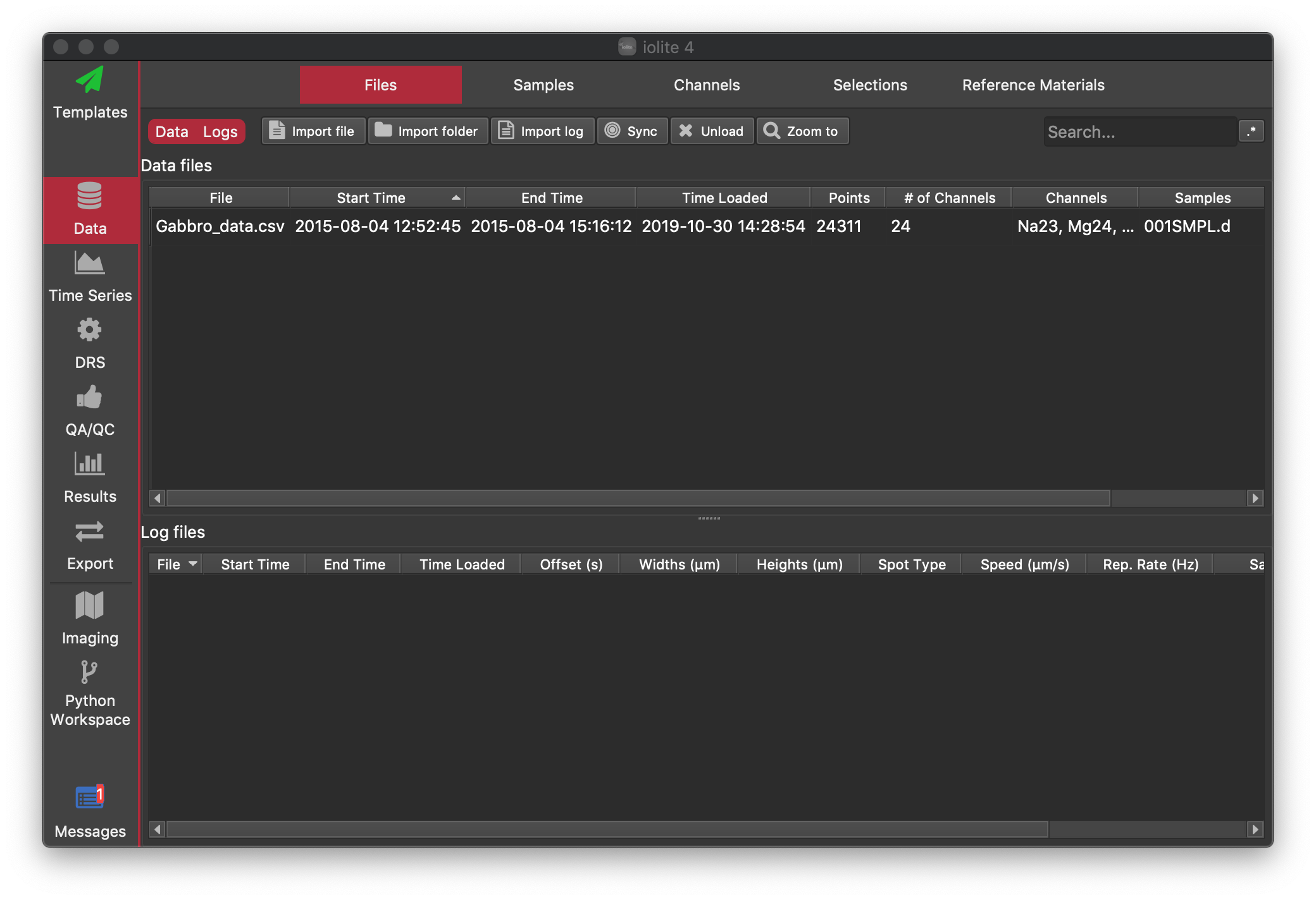
We import mass spec data by clicking the Import File button in the Data Browser, with the Files Tab selected. Select the example file called Gabbro_data.csv and click Open. You should now see that a "Data file" has been loaded (we call mass spec files "Data files" and laser log files "Log files", although both contain data). The Files Tab shows which files have been loaded, along with some information about the time interval the files contain, the channels (masses) measured and the number of data points etc. Once your mass spec data are loaded, you window should look like this:

Now let's load the laser log file. As mentioned above, the laser log file records when the laser was on vs off, the laser spot size, sample labels as well as other information. We recommend always creating laser log files with every experiment as they are very handy, but only occupy a very small amount of disc space (usually only a few hundred kB). See the Lasers section for more information about generating laser log files. If you don't have a laser log file for your own data, that's fine too. There are many ways to do things in iolite, and we'll look at some options below.

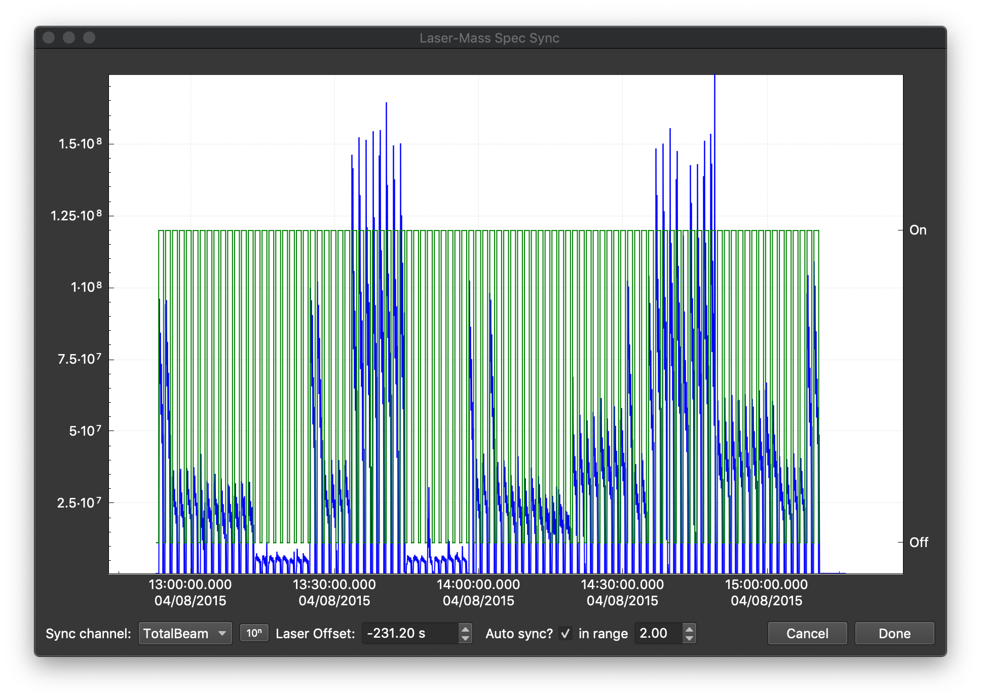
To load the laser log file, click the Import Log button. Select the Gabbro_log.csv file and click Open. This will open a 'sync window', like that shown below. This window shows the laser state from the laser log file in green. When the laser is on (firing), the green trace equals one, and where it is off, the green trace equals 0. This is plotted over the mass spec data. By default, the TotalBeam channel is shown for alignment, but you can change which channel is shown in the bottom left of the window. You can also switch between log and linear scaling for the mass spec data with the 10:sup:n button. By default, iolite tries to determine the offset automatically. You can turn this on/off using the Auto sync? checkbox at the bottom. If the autosync doesn't work, you can manually adjust the offset by holding the Shift key and clicking and dragging the green trace until it overlaps with the mass spec data. You can zoom in on the data using the mouse wheel too. When you zoom in quite a bit, you can see the individual labels from the laser log file for each spot/scan line etc. This can help you work out which part of the mass spec data to align with. For this example file the offset should be ~-231 s. Once you're happy with the offset, click on the Done button.

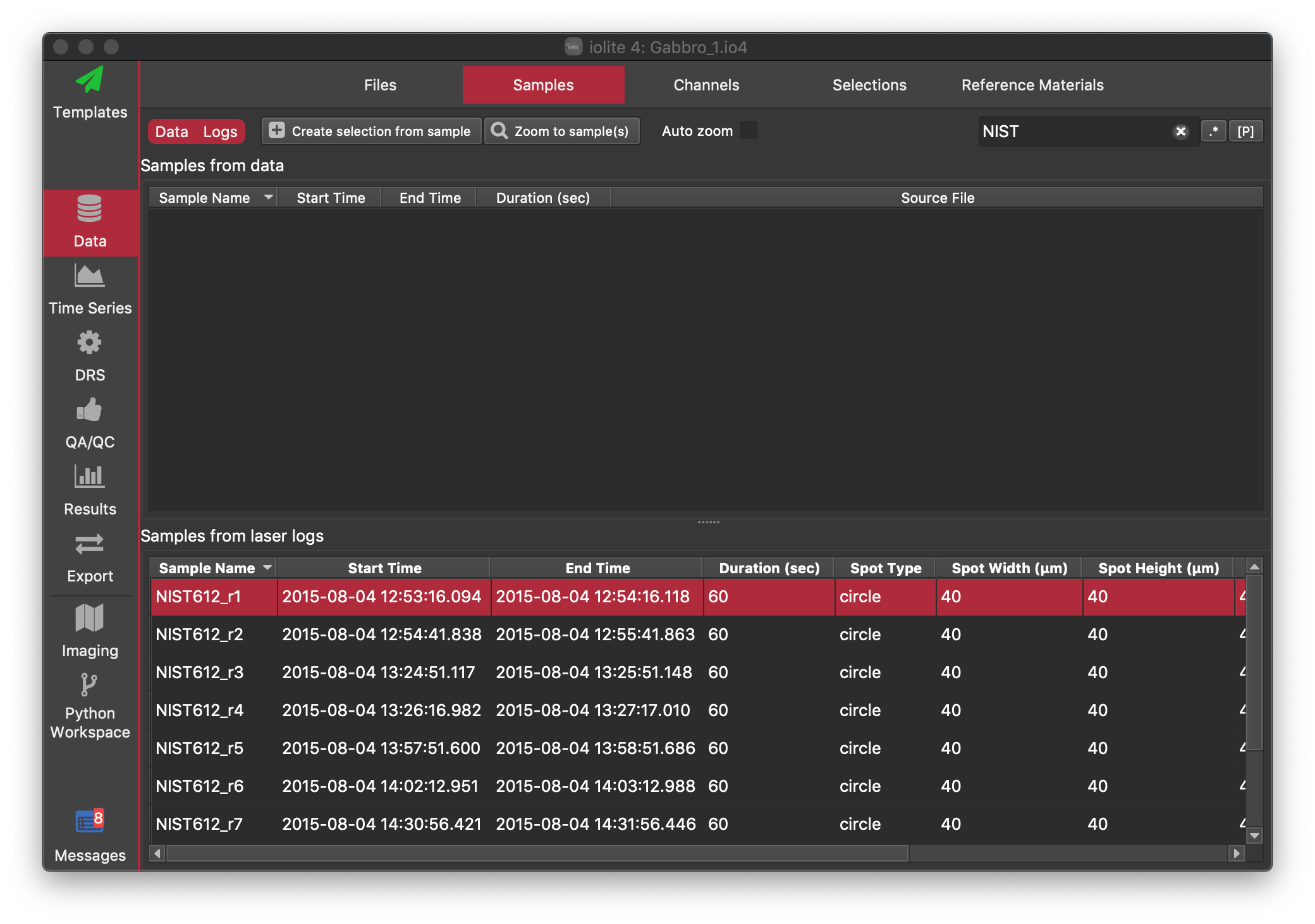
You should now be able to see the laser log file window in the Files Browser in the Log files section. If you click on the Samples Tab, you should now be able to see that there is a single Data sample (because we loaded a single Agilent file, there is always only one sample per Agilent file), and the samples that were recorded in the laser log file (e.g. NIST612_r1, BCR2G_R1 etc). Here we can quickly make selections from our samples and reference materials samples. Lets start with the NIST612 runs. We can filter the samples in the table using the Search... field at the top right. If we type "NIST" into this field, only samples with "NIST" in their labels will be shown. Give it a try. It should look like this:

To create selections from these samples, click on any sample in the list of laser log samples. Then, press Ctrl+A (Cmd+A on Mac) to select all samples. Once all of our samples are selected, we can click on the Create selection from sample button at the top. This will open a dialog to create selections, like the one shown below.

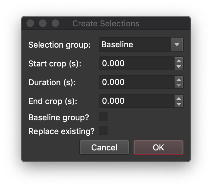
At the top of this dialog, we can select the group we want to add the selections to. For reference materials, you can just select the group name from the list, but if the group name isn't in the list, you can just type anything you like into this field for the group name. In this case, we'll select G_NIST612 from the list (if it isn't already selected). The start crop field allows us to offset the start of the selection from the start time recorded in the laser log file. Adding a positive number here will start the selection later than the start time recorded in the log file. If we wanted to set the duration of the selection, we could enter any number in the Duration field. However, because this is a laser log sample, we can just leave the duration as 0 s which will mean that the selection duration will remain the same as that recorded in the log file (± any start or end crop). We could also enter an End Crop value which would offset the selection end time to earlier than that recorded in the log file, but we'll also leave that as 0 here.

Tip

You can't set a Duration and an End Crop value, because iolite won't know whether to set the duration, or to move the selection end time in from the end time recorded in the log file. Instead, if the Duration value is anything other than 0, iolite will use the Duration value and ignore the End Crop value.

If this was a baselines group, we would check the Baselines group? checkbox, but we're not selecting baselines here, so we can just skip that. Similarly, we don't have any selections in our group yet, so we don't need to worry about the Replace Existing? checkbox either. To add the selections to the group, click the OK button.

We can now repeat the process for the BCR2G runs, by typing "BCR" in the Search... field at the top left, with the same settings as before (0 start, duration and end crop values) except that this time the selections will go into the G_BCR2G group. We can also repeat the process for the G_BHVO2G runs (using "BHVO" in the search field). We'll select our unknowns (our olivine, clinopyroxene, plagioclase etc) later. For now, let's have at look at our data and selections.

Click on the Time Series button on the left hand side of the window. This is where you can view your time-resolved data, along with your selections.

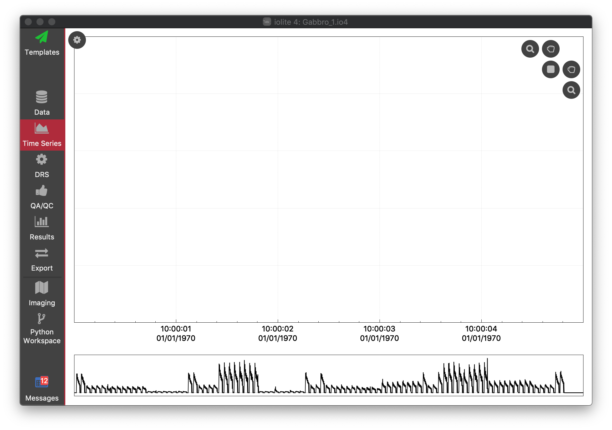
To begin with, there are no traces in the main part of the window. You can see TotalBeam vs time in the navigation plot along the bottom of the window. To add a trace to the main part of the window, open the Settings Panel by clicking the button at the top left. The Settings panel allows us to add channels to the plot, change the zoom settings, view and create selection groups, change spline types, as well as many other operations. See Time Series View for more details, but for now, let's just add Si29 to the main plot by double-clicking it in the list of channels.

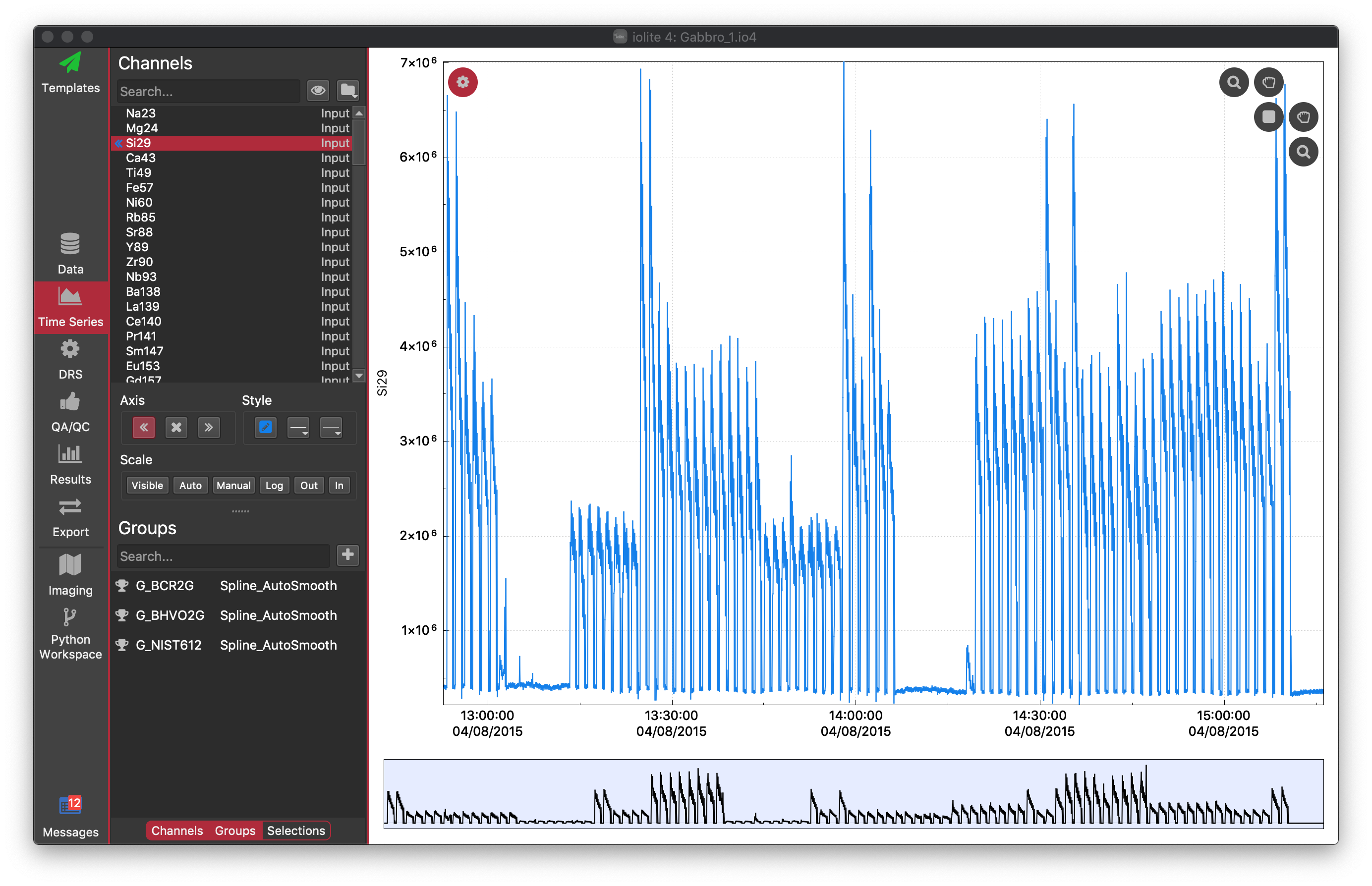
At the bottom of the Settings panel, you can see there are three buttons: Channels, Groups and Selections. Channels and Groups should already be selected. These buttons show/hide the different parts of the Settings panel. By default, the Selections part is hidden. We can leave it hidden for the time being. In the Groups section, you should be able to see the groups you created above, along with their spline type (Spline_AutoSmooth). You can click on any of these groups to show their selections in the main plot. You should be able to see that NIST612 selections have higher Si29 counts than the basalt reference materials. You should also be able to see a dashed green line going through most of the selections. This is the spline for the group.

There are many ways to create selections in iolite, but for this example we'll include how to create them manually using the baselines as an example. To start off with, we need a selection group to hold the selections. We can add a selection group by clicking the button next to the Search... field below the Groups label. It will pop open a dialog that looks like this:

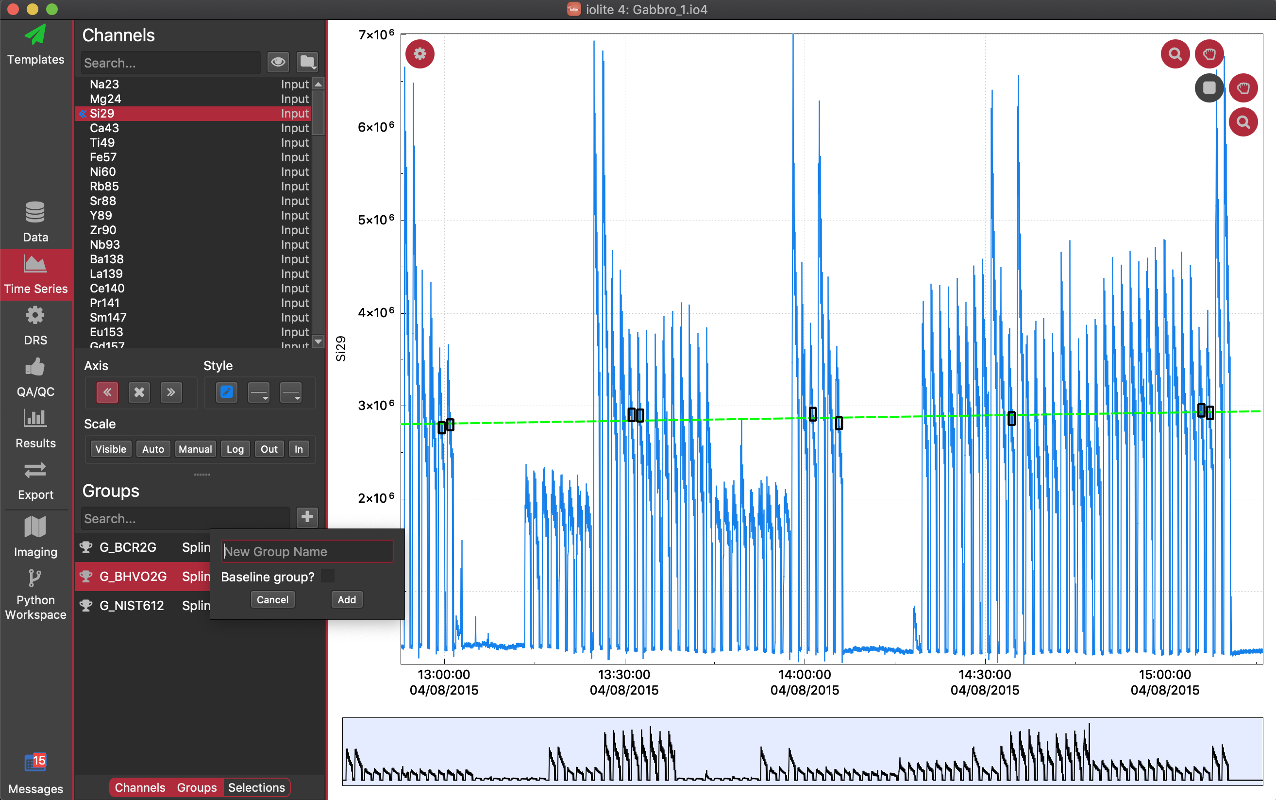
You can call the group anything but we'll call it "Baselines" just to make it obvious later on what the group contains. Make sure you check the Baseline group? checkbox, and then click the Add button. You will then see a new group has been added to the list, and that it has a different icon to indicate that this is a baselines group. Click on its name to select it. We can now manually add selections to this group, but we want to zoom in on the baselines. In the top right, there are two hand icons: one for grabbing and dragging in the horizontal axis and the other for the vertical axis. There are also two magnifying glass icons, one that allows zooming with the mouse wheel on the vertical axis, and the other for the horizontal axis. Turn each of these four icons on by clicking on them (they will turn red when on). You can now zoom in on the baseline period measured just before the first few spots.

Tip

When zooming remember that iolite will try to centre the value currently under the mouse. To ensure you zoom to the value you want, make sure that your mouse cursor remains over the data you want to zoom to.

If your data start to move off screen, you can left click and drag it to bring it back on screen (this is the effect of the grabbers being turned on).

Tip

If you want to zoom in the vertical sense only, turn off the horizontal zoom icon. Similarly, if you want to zoom in the horizontal sense only: turn off the vertical zoom icon. If you want to drag your data in the horizontal axis only, which can be quite handy when you've got a good level of zoom, turn off the vertical grab icon.

With all of this zooming and panning, you can keep track of where you are in your experiment using the navigation plot along the bottom. The blue rectangle shows the current extent of the horizontal axis in the main plot.

You can return to full data extents in the x axis by double clicking the navigation plot. You can rescale the vertical axis by clicking the Auto button in the Settings Panel. For more details on the Time Series view, see Time Series View.

Once you have zoomed in to the period before the first spot, you can create a selection manually by holding down the Ctrl key (Cmd on Mac) and left clicking and dragging to define the selection interval. Note that the selection's vertical extent is defined by the mean and two standard errors of the data within the selection. You can see this mean/uncertainty change as you select more or fewer datapoints. While the selection is in 'Edit Mode', the selection is defined by a red dashed line. While it is still in Edit Mode, you can adjust the start and ends of the selection, or you can press the 'a' key to show some more information about the selection. Click away from the selection info popup to close it.

When you click somewhere on the screen away from the selection, it will leave Edit Mode. When a selection is not in edit mode, it will be defined by a solid black line, and you can't adjust it.

Zoom to the other end of the experiment and add another baseline selection manually. Click away from the selection to leave Edit Mode.

Note

We're just going to add two baseline selections in this tutorial. Normally you would add as many as needed to accurately define your baselines. You should always check each channel to make sure the baseline spline goes through the baseline data.

Now we an go back and select the unknowns for this experiment. It's easiest to do this using the Samples Browser just as we did for the NIST612, BCR2G and BHVO2G selections. You can type the following into the Search... field to select each mineral type: 'Oliv', 'Plag', 'Opaq', 'Cpx'. You can either put them all in their own selection group, or you can put them all in a single group. Using a new group for each mineral will just make it easier to view the results later on. Once you've done that, we can run the Trace Elements DRS.

Click on the DRS tab on the left side of the window. Select the Trace Elements DRS from the list on the left. This will show the Trace Elements DRS settings.

Note

For those who have used iolite v3 in the past, iolite v4 combines the Trace_Elements and Trace_Elements_IS Data Reduction Schemes (DRS) into a single DRS.

In iolite v4, you can set different reference materials for different channels. For example, using NIST612 to calibrate Ti49 might not be as accurate as there is very little Ti in NIST612. However, for this example, we're just going to use NIST612 for everything and observe the results. To set the reference material for all channels, click on a channel name in the list of channels to select one of the channels. Then press Ctrl + a (Cmd + a on Mac) to select all channels. Then click on the Set Ref Mat button at the top of the channel list, and select G_NIST612 from the list of options.

In this example, we're going to use internal standards (IS) (as we're processing spot data), but if we didn't want to use an IS, we could uncheck the Use Internal Standards checkbox at the top of the settings. If this is unchecked, the IS table on the right is disabled. We are going to use an IS, so make sure it's checked. The Internal Standards Table occupies the right half of the settings. We can use this table to type in the channel (element) to use for each selection, along with the value to use, and the units of each value. However, typing it in would take a long time for most experiments, so you can load a text file containing IS values. You can also copy the table to Excel, and paste values from Excel directly into this table. To load our file containing IS values, click on the Import IS values button at the top of the Internal Standards Table.

We're going to load an IS table file. This is just a tab-delimited text file that has the selection labels in the first column, and IS data in the other columns. In our example dataset gabbros_example_data.zip that you downloaded at the start of the tutorial, there is a file called Gabbro_IS_values.txt. This file contains the selection labels in the first column, and the Ca wt % for each grain (measured by EMPA) and the Ti wt % for each grain as well. We can load this file by clicking the Load IS Table button at the top of the settings. We can select our .txt file and click Open. It will appear that nothing has happened, but in fact iolite has matched the labels in the file to selections and stored the Ca and Ti values as properties of the selection. This way, we can change between Ca and Ti as our IS and not have to reload the file each time. Now, if we select all selections in the table byclicking on one selection and then pressing Ctrl + a (or Cmd + a on Mac) and then click on the Element button at the top, and select Ca43, iolite will populate the table with the Ca values we just loaded. It will also automatically load the Ca values for our reference materials. By default the units will be set to wt %, but if you have used different units, you can set them now using the Units button. If we didn't have an IS data file, and we wanted to set all selections to have the same IS value, we would select them all, set the element using the Element button, and set the IS value for all using the Value button and typing in a value.

Now that we have set the IS values, and external reference materials, we can "crunch" the data. "Crunch" here just means to run the DRS. The DRS is a set of instructions that processes your data from raw data to final results.

Tip

Running the DRS does not change any input data, so you can crunch the DRS as many times as you like.

The DRS will perform as many steps as it can until it either finishes sucessfully, or finds that it needs more information. For example, if you haven't selected any reference materials, the DRS will continue up to the point where it would calibrate using the reference materials and let you know that you need to make some selections for it to go any further.

Tip

Sometimes you might actually want to partially run a DRS. You can generate intermediate channels such as raw ratios and use them to make automatic selections.

Click the red "Crunch" button at the bottom left to run the DRS. You should see a progress indicator in the bottom right of the window. The DRS should run to completion, and you now have final (in this case ppm) channels. You can then use iolite's visualisation features to check your results, or run a QAQC module to check your results before export, or before creating images etc. In this case, we'll check our secondary reference materials.

Click on the Results button to show the Results View. The Results View has three tabs: Summary Stats, XY Plot, and Data Table. The Summary Stats view shows summary stats for each selection group in a table at the top and a plot of the mean ± 2SE for each selection in the bottom half of the window. The XY plot is very similar, with summary stats for two channels at the top and you can plot two channels, one on the x axis and the other on the y axis to show relationships between channels. The Data Table tab shows the mean ± 2SE for each selection for each channel in a table. You can select which channels are shown and filter the table in many different ways, but for the time being, we'll just use the Summary Stats tab to check our results.

We'll begin by showing the results for BCR2G by clicking on the checkbox to the left of it's name in the table. The checkbox may be hard to see, but if you click to the immediate left of the name, you should see a check appear. This will plot the Na23 results in the bottom half of the window (the input channel). We can check the output (ppm) channels by selecting one from the Channel selector in the right top part of the window. Let's select the Sr88_ppm channel from the list of Output channels. Iolite will plot the selection means and 2SE in the bottom half of the window, and the tabl will show the mean, uncertainty, number of outliers etc for each selection group. This gives us an average for each group, which is better than comparing a single selection to the accepted value. In this case, you should get an average Sr88_ppm value of around 328 ppm for the BCR2G group. If we go to the Reference Material browser (in the Data View), you can click on the Data tab, you can see that the accepted value (at the time of writing) for Sr in BCR2G is 342 ppm. So, our average value is a little low. You can see in the bottom half of the Summary Stats window that this is because of the third BCR2G run. It is lower than the rest. We can double-click on this selection to see if there is something odd about the Sr results.

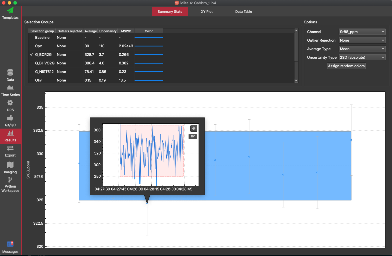
From the popup, which shows the time series for the selected channel (in this case Sr88_ppm), we can see that there is nothing obvious about this ablation to warrant its deletion. If there was a drill through etc, it might be obvious in this popup, although we might want to go back to the Time Series View to do some more investigating. In this case, it's just analytical noise, and even if we use outlier rejection to remove this result (using the Outlier Rejection selector in the top right, under the Channel selector), it wouldn't change the average value by much. The difference here is more likely due to calibrating a basaltic glass with a NIST glass, as there might be matrix effects. The offset here is acceptable, and we can go through our other channels to check how our secondary reference materials performed.

Tip

We always recommend checking secondary reference material results. They are treated in the same way as unknowns (unlike the primary reference material selected in the DRS settings window), and so they are a good independent test of the entire data reduction process.

It can be a little slow to check each channel against its accepted value manually in this way. If we want an overview of how the group average for each channel compares to the accepted value, we can use the built in QAQC module "Secondary Check".

Quality Assurance/Quality Control (QAQC) is basically just checking your data against accepted values. So basic QAQC modules are built into iolite v4, but you can write your own. Here, we're going to use the "Secondary Check" QAQC module. This module compares the result for each channel to the accepted value for a selected reference material. Click on the QA/QC button on the left hand side of the window to open the QAQC View. On the left of the View, you'll see a list of available QAQC modules ("Element Check", "Z Score" etc). Double click on the Secondary Check item to open this module in the main part of the View. You can have multiple QAQC modules open at the same time, and their windows can be minimised, maximised etc using the buttons in the top right of the module window.

Each QAQC module has a Settings button in the top left. Click on this button to open the settings panel.

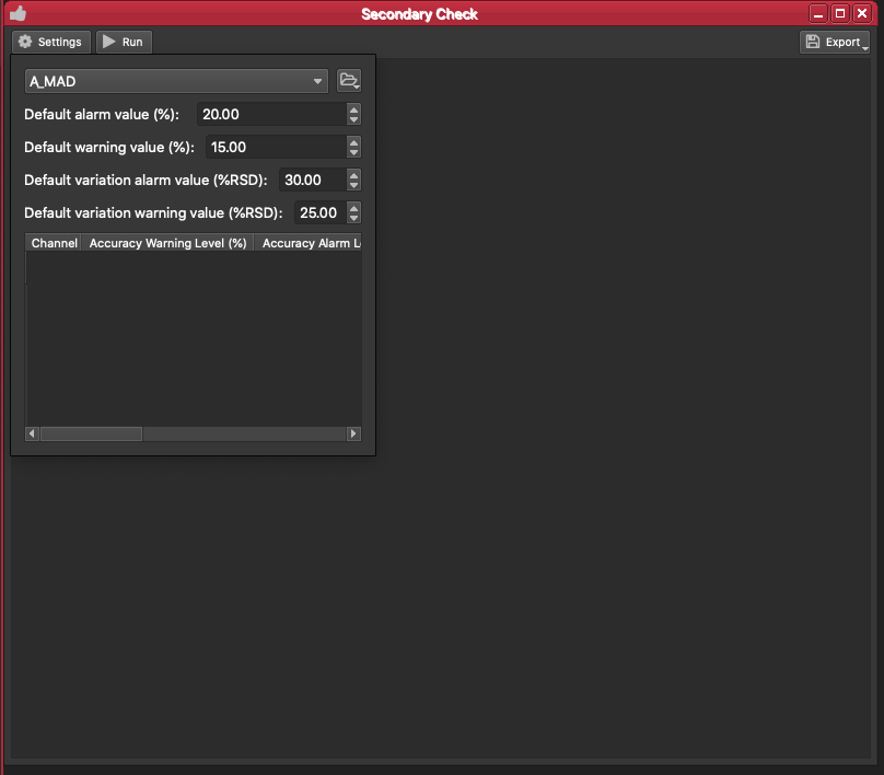
At the top of the settings there is a dropdown menu to select the reference material you want to view results for. Select G_BCR2G. iolite will then create a report, including a graph and table, showing the mean result for all analyses of this reference material compared to the accepted result (you can see the accepted values for a reference material in the Reference Materials Browser).

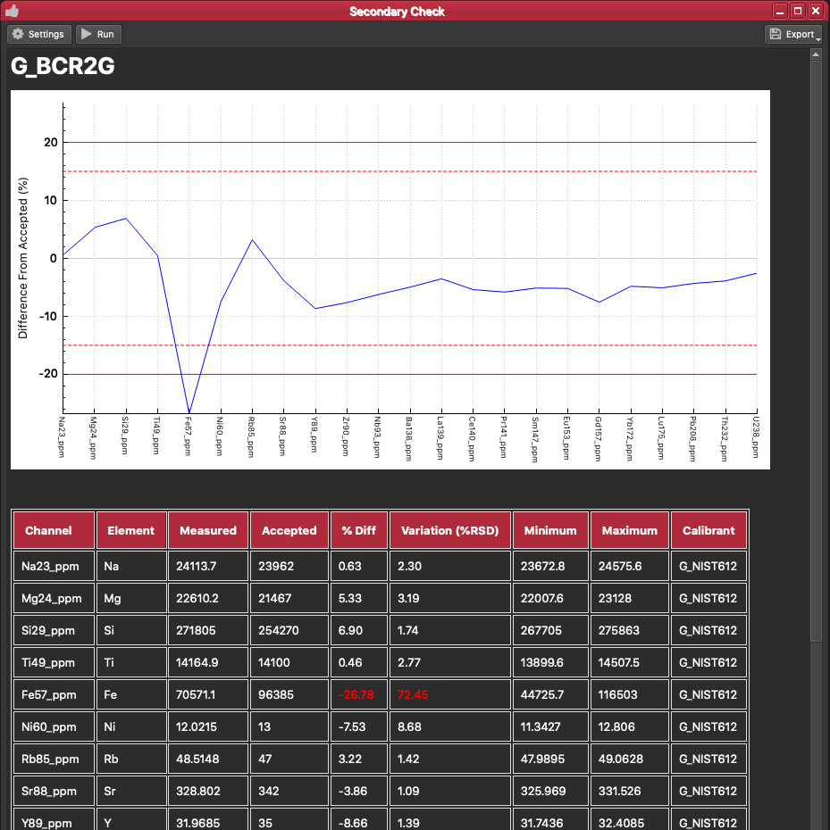
The graph shows how the mean value for each channel differs from the accepted value. There are also four red lines across the graph: two dashed lines, and two solid lines. These lines represent Warnings and Alarms. A Warning is a threshold beyond which iolite will issue a warning that a result is beyond the Warning value. By default this Warning threshold is 15%. This means that if the mean result for a particular channel (e.g. Fe57_ppm) deviates by more than 15%, iolite will record a Warning. An Alarm is a similar threshold, beyond which iolite will issue an Alarm. Alarms can be used to halt automated processes such as Processing Templates etc. Both Alarms and Warnings are recorded in the Messages log. You can see these Warning and Alert thresholds in the graph as dashed red lines (Warning threshold) and solid red lines (Alarm threshold). You can set the thresholds for Alarms and Warnings in the Settings panel for the QAQC module.

The QAQC report table shows the mean result for each element ("Measured") along with the accepted value, and the percent difference. The table also shows how much variation there is within the group as %RSD. You can also set Variation Warnings and Alarms, similar to described above. These work on issuing an Alarm or Warning if the varation of a group is beyond a certain threshold, so that you can also see if your results have the correct mean (i.e. low % difference) but are quite scattered (high %RSD).

You can save this report (as HTML or PDF) using the Export button in the top right. You can also highlight the graph and/or table and copy and paste it to the Notes panel, or to other applications. Once you have checked all your secondary reference materials (G_BCR2G and G_BHVO2G in this example), and you are happy with the results, you can continue to inspect your results, or you can export your data.

To export your data, click on the Export button on the left side of the main window. Initially, this will show your favourite export configurations. You may not have any yet, so click on the Export to File button at the top to export your data to an Excel or csv file.

Tip

You can also use python scripts to export your data, or use scripts written by others. This allows you to export your data in any format you wish. Please see https://github.com/iolite-LA-ICP-MS/iolite4-python-examples/tree/master/export for a couple of examples.

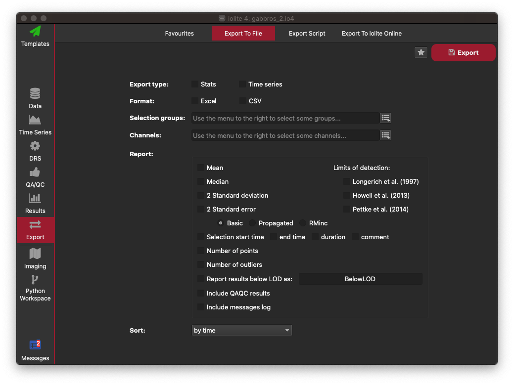
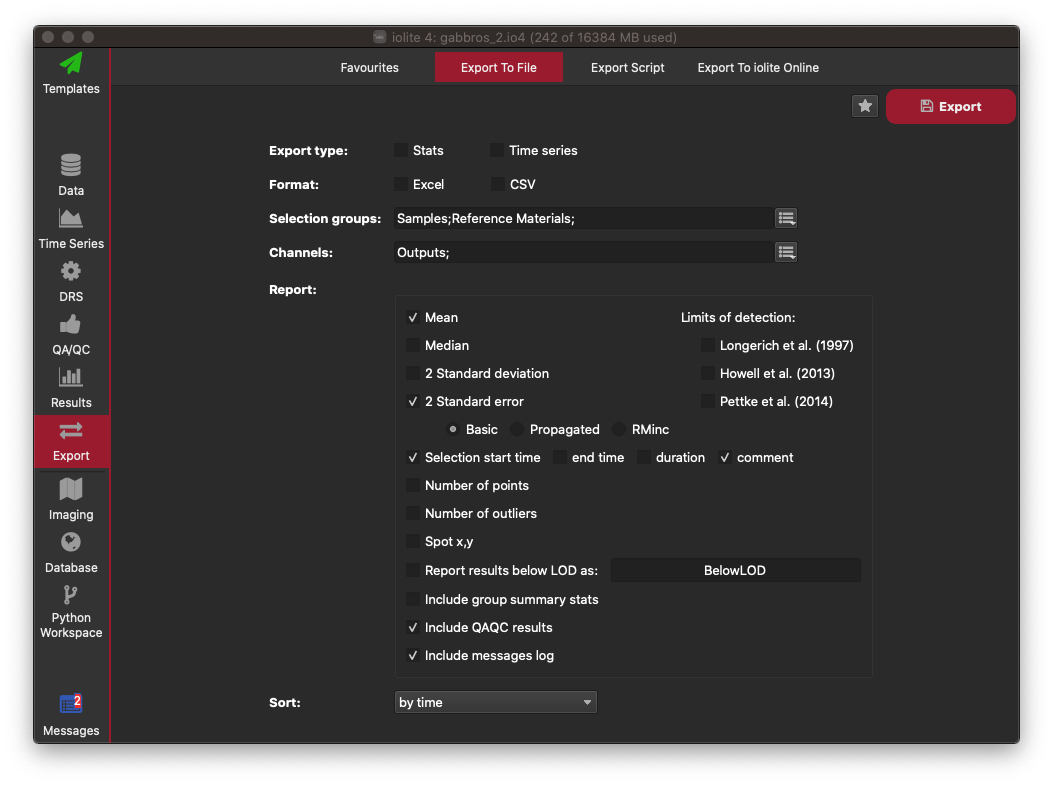
Here you can select whether you want to export an average for each selection ("Stats") or the data within each selection's interval for all channels ("Time series"). Most often you'll want to select the Stats option. You can then choose the export format: Excel in this example. Select which groups you want to export values for using the button to the right of where is says "Selection Groups". In this example select Samples and Reference Materials to export all non-baseline groups. In the channels selector, choose Outputs. Then in the options for what to report for each channel, click Mean, 2 Standard Error (basic), Selection Start Time, Comment, Include QAQC results, and Include messages log. An image showing what your configuration (in this example) should look like is shown below. You can now click on the star icon in the top right to save this as an Export Configuration. The next time you want to export your data, you can use this configuration to save you having to re-select all these options. Give your configuration any name e.g. "Basic Export" and click OK. Now click the Export button on the top right to export your data. Select the filename and folder where you want to save your file, and click Save. A panel will appear along the bottom of the iolite window with an Open File and Open Folder button. Click the Open File button to open the file you just created. This will start Excel. You will now be able to see all your results, along with your QAQC data, metadata, and processing log.

This concludes this very basic tutorial. Please note that many parts (if not most) of this process can be automated, either by using a Processing Template, or other tools within iolite.

There is more information about many of the concepts covered briefly in this tutorial in the User Interface Guide. For example, more detail about using internal standards and calculating LODs is avilable here.

Note

If you have any questions or comments about this tutorial, please see the dedicated forum post here