Imaging

This is a step-by-step guide to image creation and interrogation using iolite v4. You should have already read installed iolite v4 before beginning this tutorial.

To follow along, you can download the examples files here.

The example files include:

Otolith.csv:

An Agilent mass spectrometer data file, format dd MM yyyy hh mm ss.

Otolith_log.csv:

A laser log file, describing the name of each ablation spot, when it started and ended and its x,y location and more.

Otolith_MAPPED.png:

An image file of the otolith, coordinated in the laser ablation software.

Otolith.coord:

An xml file describing how the image is coordinated into cell space.

This data set was not intended to be fully quantitative and therefore only includes a few measurements of NIST612 and no QA/QC measurements. The image or map was acquired while rastering a 93 μm circular spot firing at 5 Hz and scanning at 30 μm/s over an otolith. A limited selection of analytes were included: 25Mg, 31P, 43Ca, 63Cu, 88Sr, 138Ba, 208Pb, 232Th, and 238U.

Loading the data

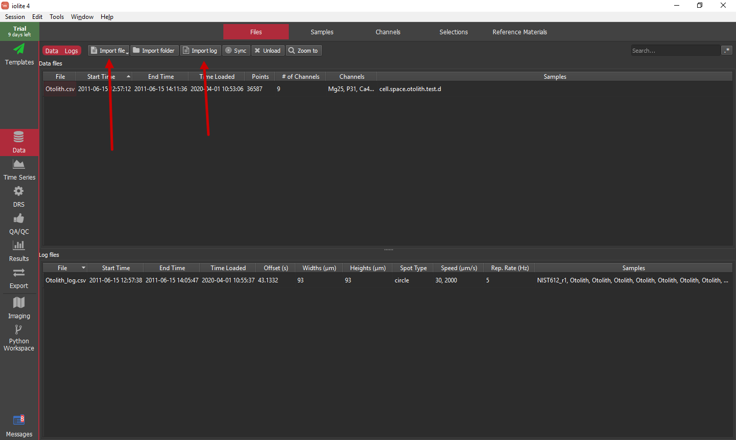
To begin, start a new session either from the welcome window or the Session ‣ New Session menu item. Next, import the raw data file (Otolith.csv) and the laser log (Otolith_log.csv) using the buttons highlighted below.

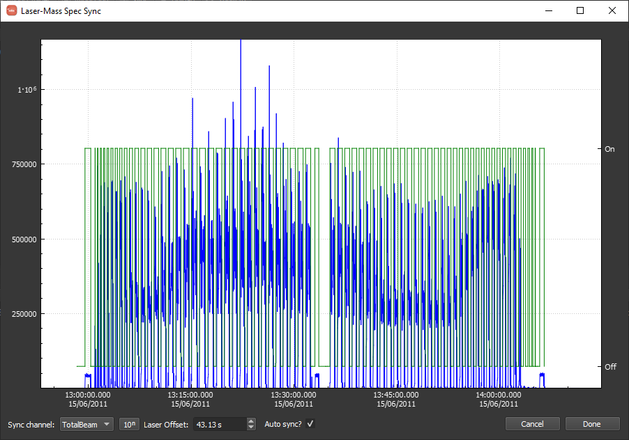
The laser log synchronization window should look approximately as below with a laser offset of ~43.13 s calculated automatically. If the offset is different, perhaps the Agilent data file was imported with the wrong date-time format. It really does not matter as long as the data and the log appear synchronized. This can be verified by using the mouse wheel or track pad to zoom into the plot combined with clicking and dragging to pan the view as needed. If the synchronization needs to be adjusted manually you can uncheck "Auto Sync?" and shift-click and drag to move the log relative to the data. When you are happy, click "Done".

Setting up selections

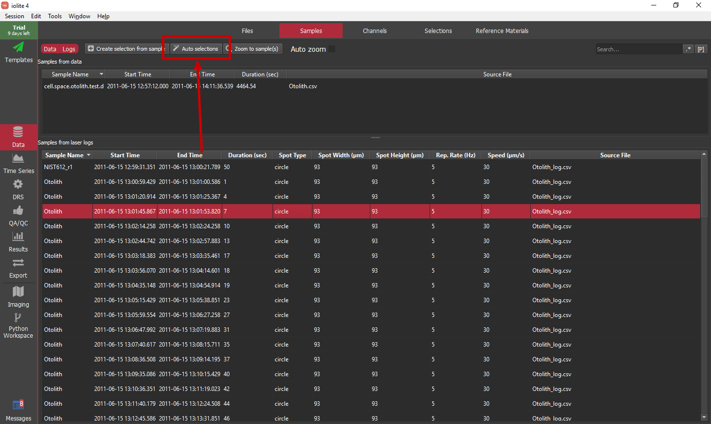
For this tutorial we will use the easiest approach to setting up selections, which is to use the "Auto Selections" button highlighted below.

Hint

Be sure to click in the Samples from laser log table before clicking the "Auto Selections" button for the routine to use the laser log samples as opposed to the data file samples.

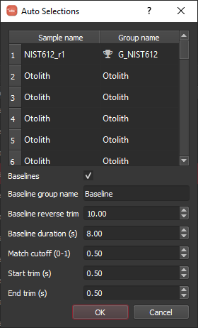
When you click the button, you will be presented with a dialog as shown below. This allows you to verify the sample to group assignments that were determined automatically. A match cutoff of 0.5 seems to work fine for this example and the various trim and baseline parameters can be setup as shown.

Note

The experiment had time between each line of the image where background was collected. This allows us to use the laser log samples to automatically setup background selections. The parameters shown will go back 10 seconds from the start of each line and create a baseline selection of 8 seconds duration.

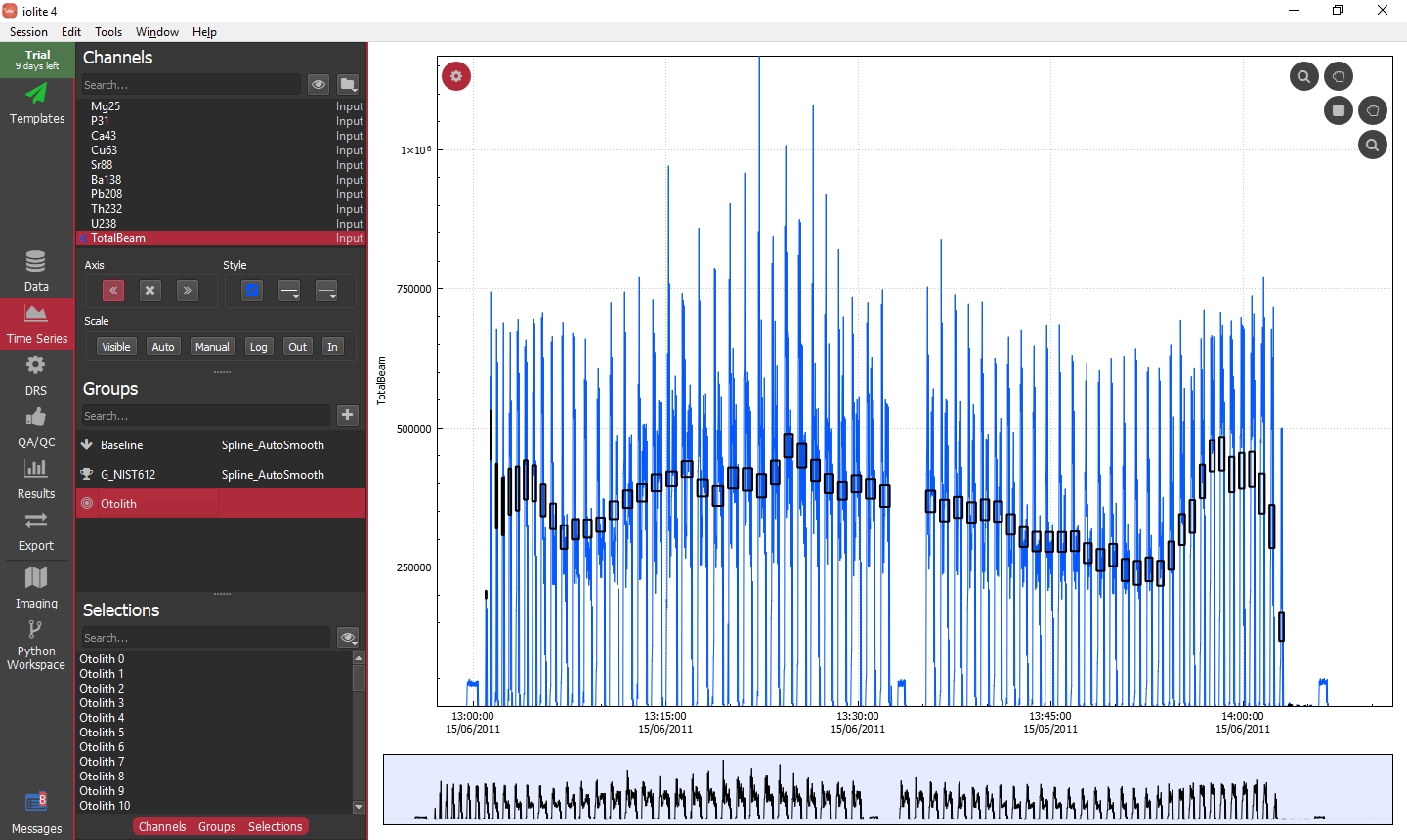
Finally, to be sure everything was setup correctly, we can go to the Time Series view and have a look at how the selections match up with the data.

Running the data reduction scheme

With our selections setup, we can now run a data reduction scheme to convert our input data into concentrations. In this example, we will stick with a semi-quantitative approach and use NIST612 as our external standard for all analytes. The setup is shown below with a few notable changes from the defaults highlighted.

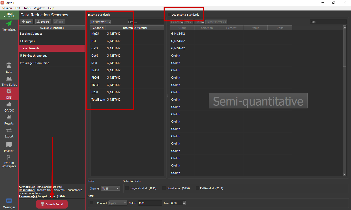
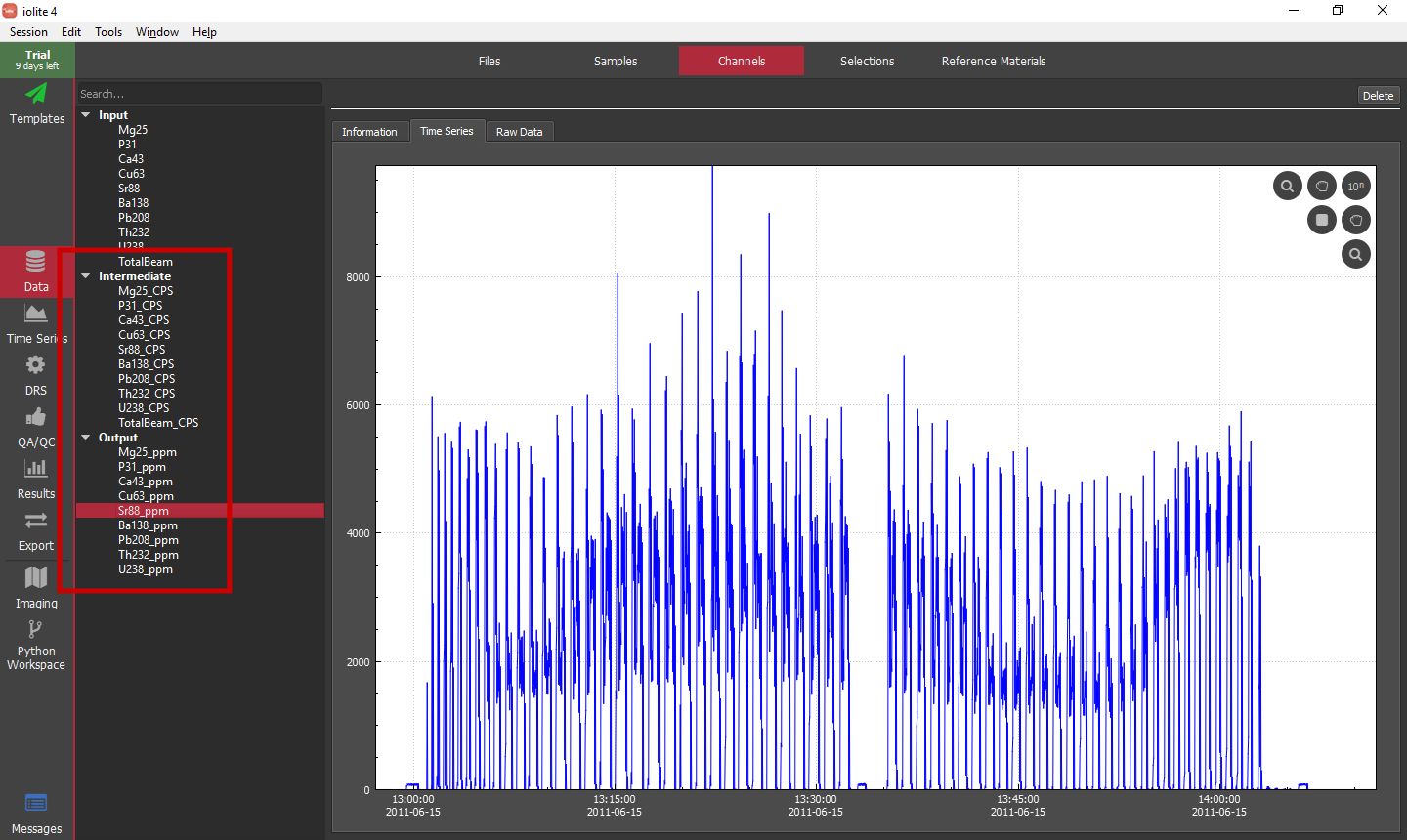
Once things are setup, simply click the big red Crunch Data! button to calculate our time-resolved concentrations. We can go to the Channels Browser within the Data view to see the newly created channels (or the Time Series view). For this setup we will have Intermediate channels with '_CPS' suffixes that are the baseline subtracted versions of all of the input channels, and Output channels with '_ppm' suffixes that are the semi-quantitative concentrations of each of the inputs.

Note

We did not inspect how our splines look in the time series view before running the data reduction scheme. By default the baseline and reference materials will use a spline with automatic smoothing to interpolate between their measurements. However, since we only have 3 measurements of NIST612, it will default to linear interpolation between the measurements as so few measurements are insufficient to construct a true spline.

Creating some images

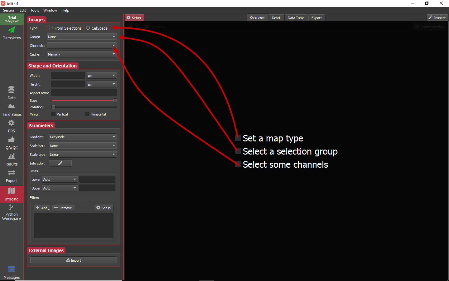
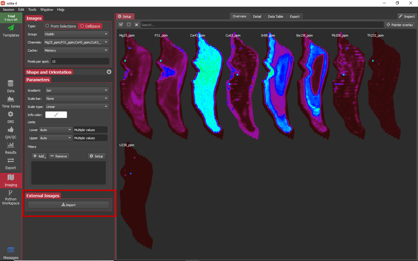
When we first go to the imaging view by selecting it on the left side panel we will see a list of things we need to set before images will be created. These tasks and where to set them are highlighted in the image below.

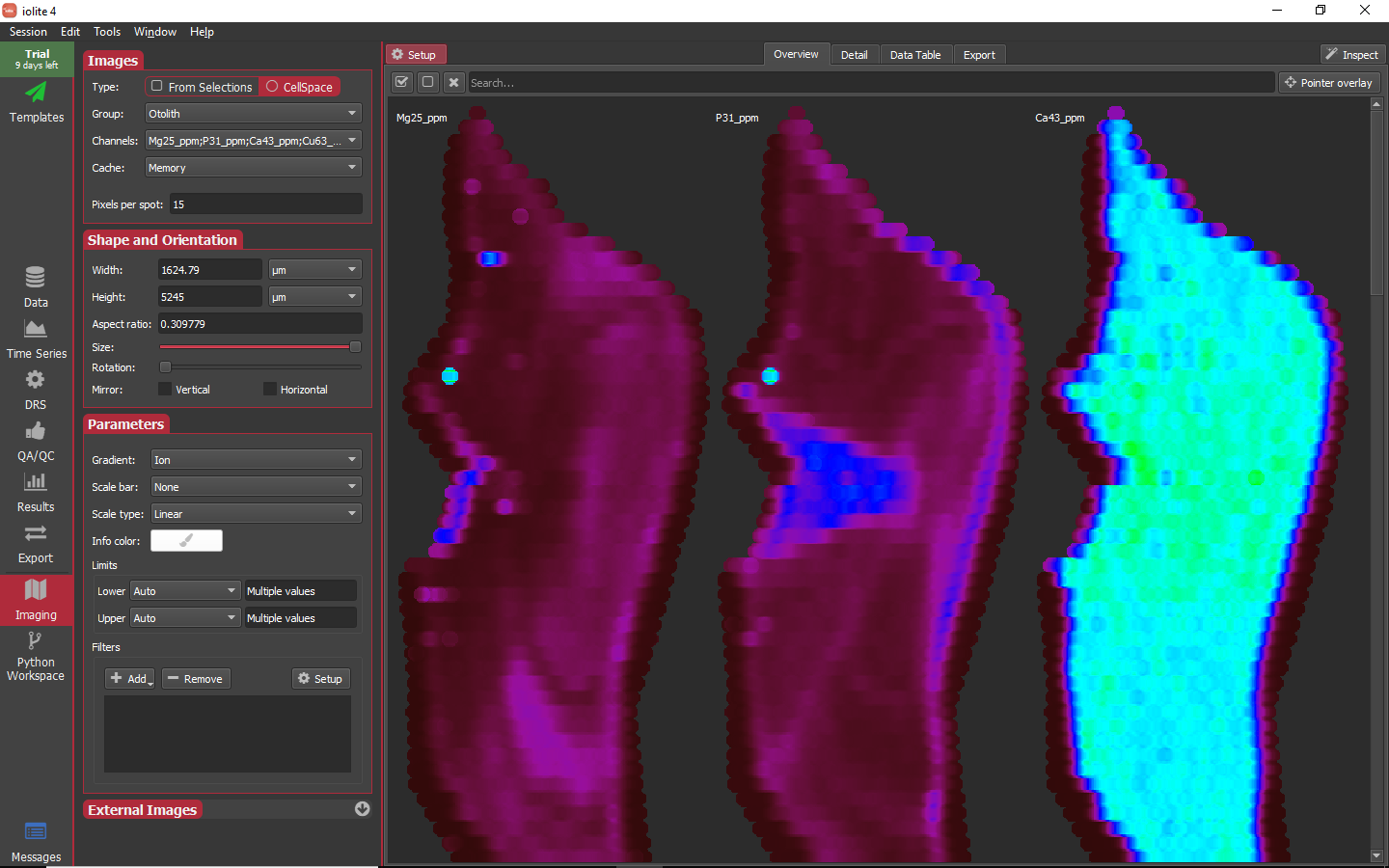
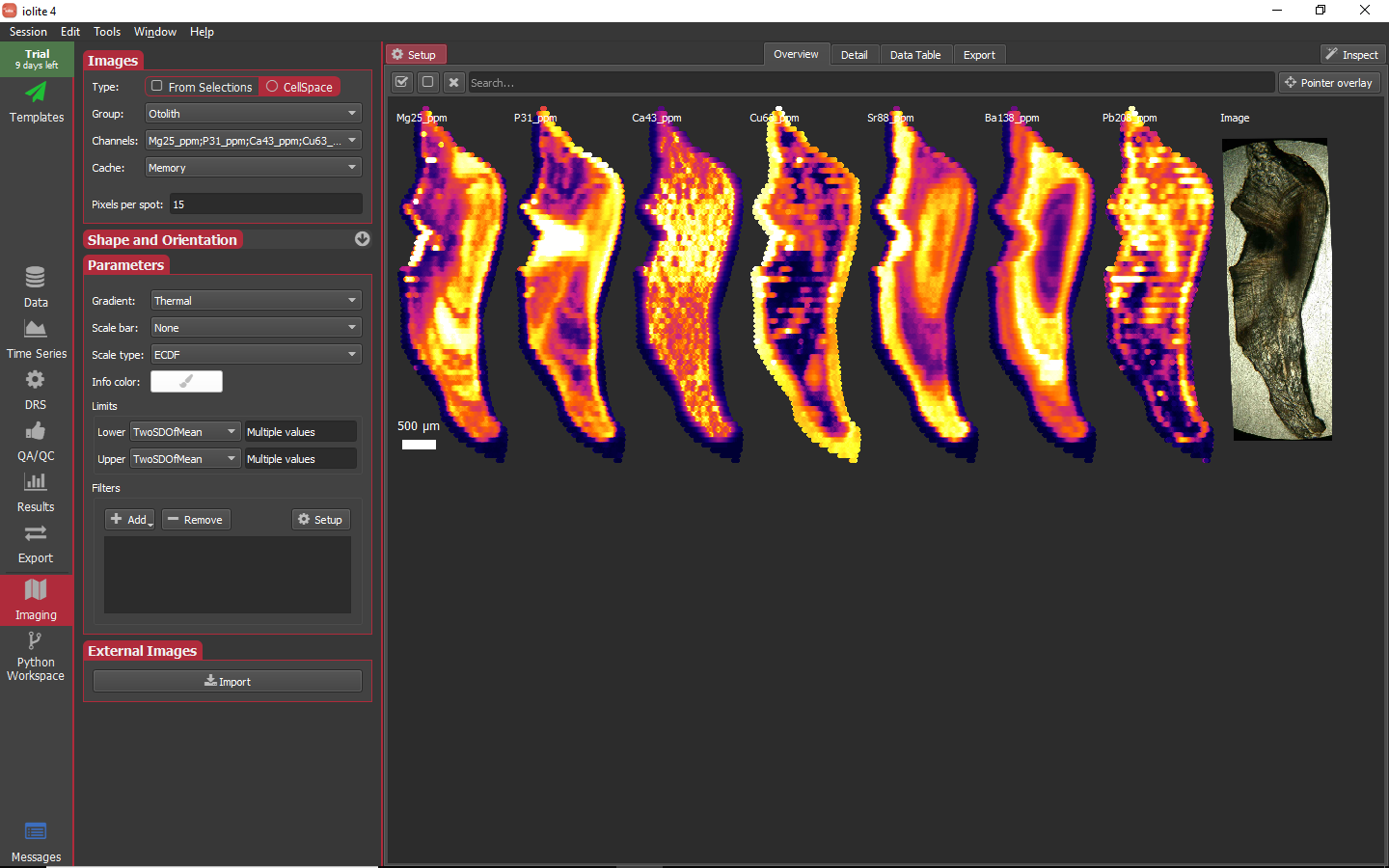
Since we used a laser log to set up this session and the selections are not equal length or aligned in any way, we will set the type to CellSpace by clicking on that option. Next, in this session we only have one group that was an image (Otolith), so we will select that as the group to map. Lastly, we will select all the output channels as the channels to construct maps for. In doing so, the imaging view should look roughly as below.

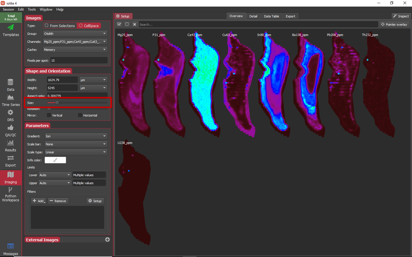
The overview images by default may seem a bit too large (or too small). You can adjust the size of each image in the overview by changing the Size slider highlighted below.

Hint

When dealing with a lot of images and/or high resolution images and/or a limited resource computer, you may want to consider changing the pixels per spot setting. This tells cell space how many pixels to represent each spot with. For circles, a higher number of pixels per spot will have the representation be smoother. For rectangular spots, the resolution is less important unless you want to capture small scale spot overlap.

Hint

Each sub-panel of the imaging setup area can be collapsed/expanded by clicking on the title.

Bringing in external images

For this data set we have a coordinated image captured with the laser software. We can import this image to be displayed along with our other images by clicking the button highlighted below.

When you click the Import button, a file chooser dialog will ask you to select an image. For this example, navigate to the Otolith_MAPPED.png available above. In doing so, a new dialog will appear to align the image to the data.

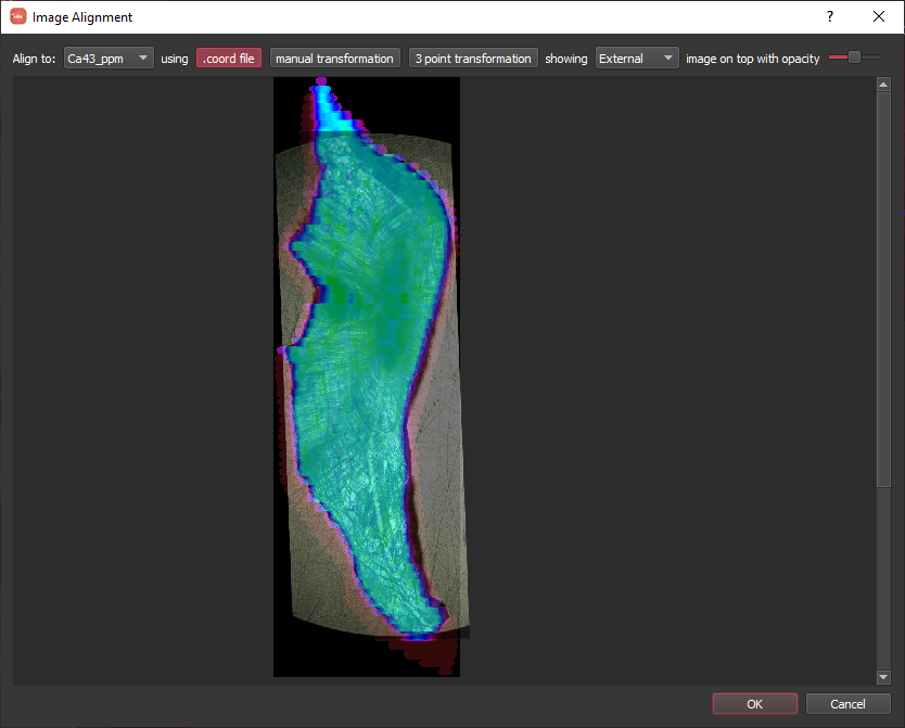
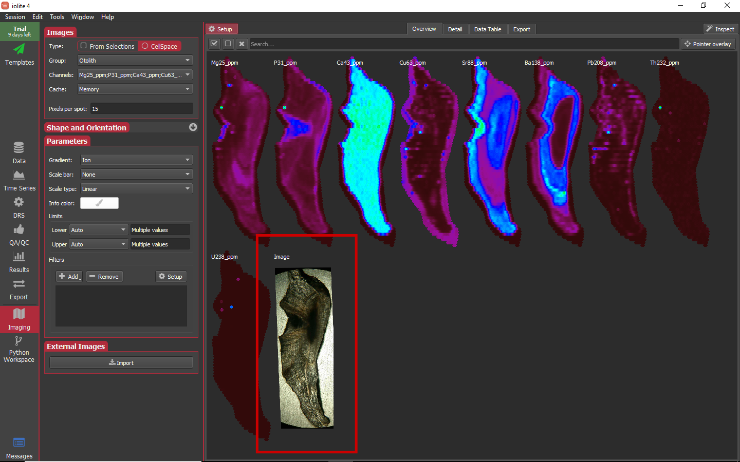
Our Otolith_MAPPED.png has an associated Otolith.coord file that will be found automatically and used to translate the image into cell coordinates (i.e. compatible with the coordinates in the laser log file). The dialog will show the image with transparency on top of one of the image channels. Once you are happy with the alignment, click OK. Now you will be presented with a dialog to name the new image. This can be anything you like, but for this tutorial it will simply be called "Image". Once it is named, it will be shown along with the other images in the overview.

Hint

Using a .coord file seems to provide the best results. However, if you did not have a .coord file, a 3 point transformation can be fairly accurate if you have sharp features you can match between the data and your image. Use manual transformation as a last resort.

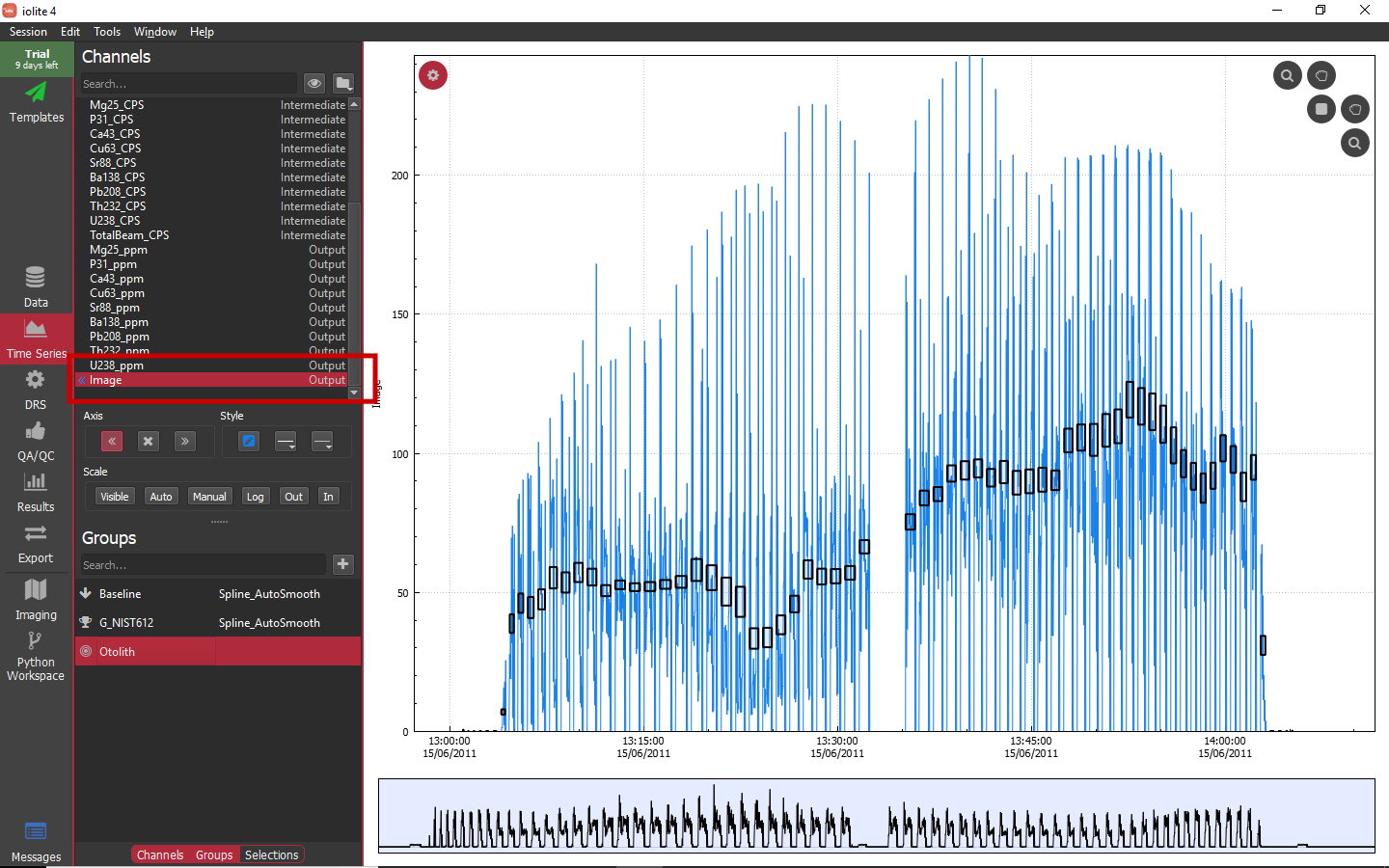
When external images are imported into iolite, the greyscale intensities of the image corresponding to the channel data is converted into a regular iolite channel named as above. For example, see below where there is now an output channel named Image with values ranging from 0 to 255. As this is a channel like any other in iolite, you can use it like any other channel and also get results for it it.

Adjusting image presentation

One of the first tasks to tackle in imaging is to choose which images to keep and how to scale and augment them. To remove an image you can go to the channels selector and toggle it off or click on the image to remove to select it and then click the X button just below the Setup button. For this data set there does not appear to be anything to see in the Th and U images, so we can discard them. Adjusting the visualization of the images is mostly done in the Parameters sub-panel. One possible set of parameters is shown below where I have adjusted the color gradient to be thermal, set a scale 500 μm scale bar on one image, set the lower limits to 0 and upper limits to be TwoSDOfMean.

Hint

When no images are selected, changes made to the parameters are applied to all images. When one or more images are selected, changes made are only applied to those images.

Hint

If you have a lot of images (e.g. from TOF data) finding an image in the overview can be tricky. If you are having trouble finding an image, use the Search... field at the top of the overview.

Adjusting the presentation of images is a matter of personal preference, so we will not make any further changes.

Looking in more detail

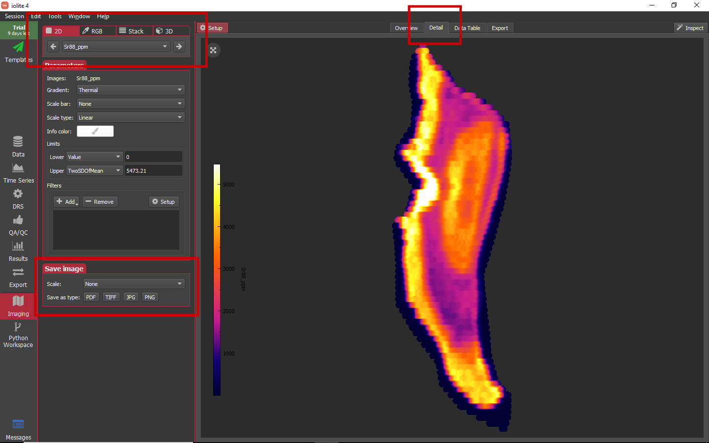
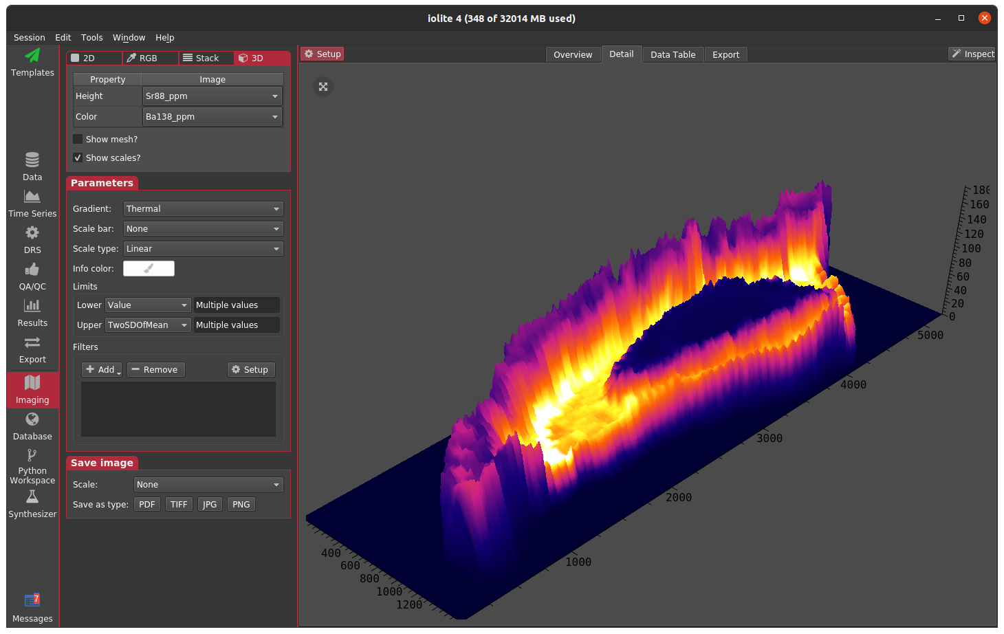
So far we have worked only in the Overview tab of the Imaging view. Next we will look at Detail tab. This is an area that allows you to look at images in more detail via larger views (2D) or combining images to provide a different perspective (RGB, Stack, and 3D). To switch between these different Detail modes, you can click the buttons along the top of the left Setup panel when in the Detail tab. The mode specific settings show up immediately below the mode selector. Below that are the Parameters and Save image sub-panels. The Parameters sub-panel is familiar from the Overview tab, and the Save image sub-panel allows you to easily save a detailed image. The Detail tab, detail mode selector, and Save image sub-panels are highlighted in the image below.

Hint

Each of the detail views has a round button in the upper left corner of the plotting area that allows you to center and resize the image to fit.

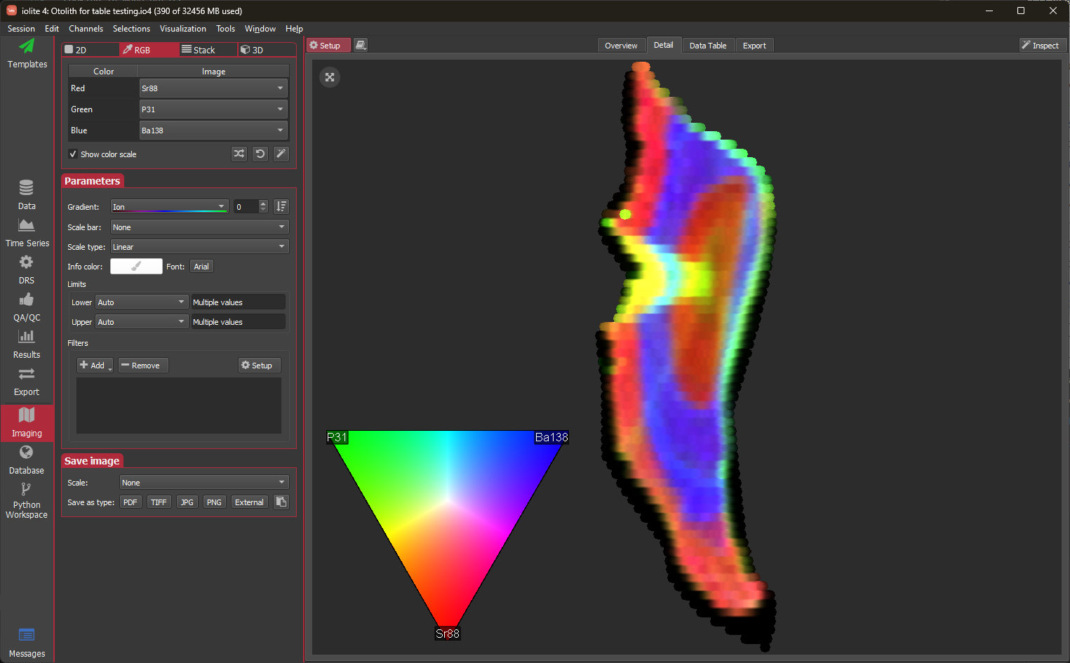
The RGB mode allows you to pick images to represent red, blue and green to be combined into one RGB image.

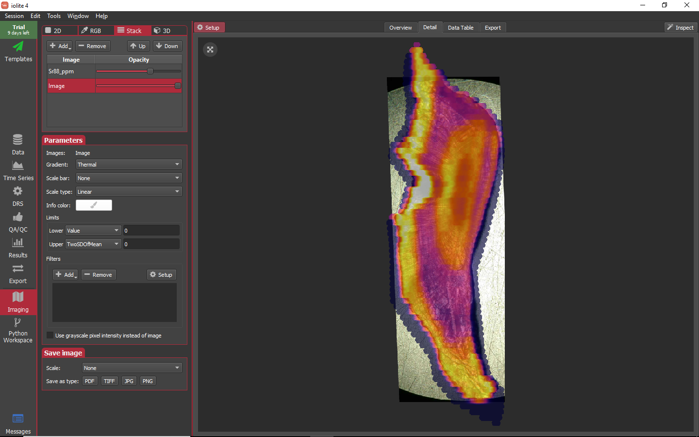
The Stack mode allows two or more channels to be blended with transparency.

Lastly, the 3D mode allows one channel to be assigned to height and another to color.

Each of these modes can be helpful when trying to visualize relationships between two or more channels.

Interrogating the image

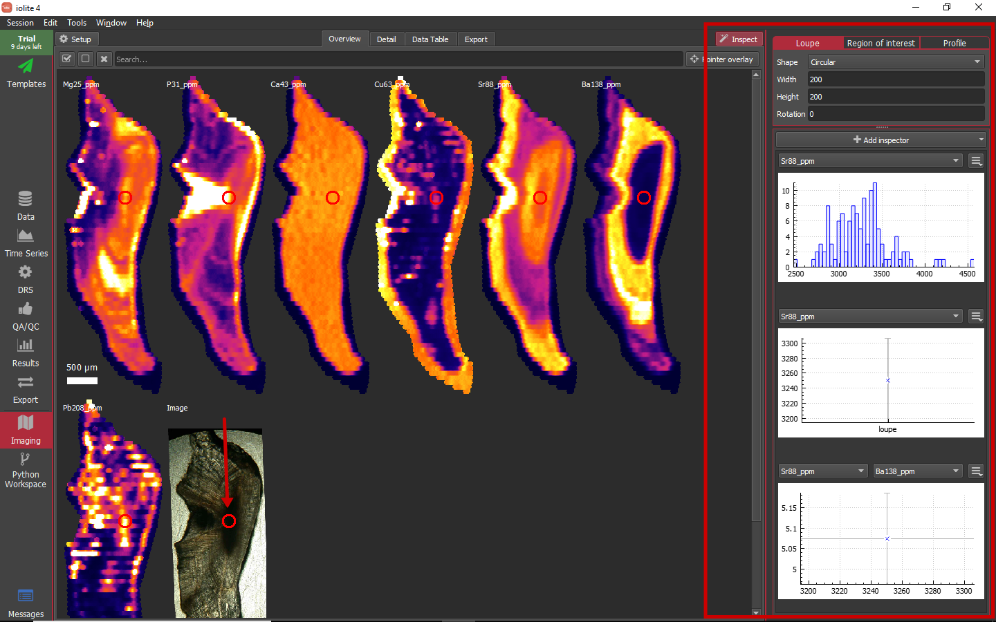
When you expand the Inspect panel on the right side of the imaging view, you will be presented with 3 different tools that are selectable along the top. These tools are: Loupe, Region of interest and Profile. Beneath the tool selection region at the top right, there is a panel that allows you to add various inspectors. These inspectors range from simple statistical plots to concordia diagrams. When using the Loupe tool, the data encapsulated by the loupe is what is used for the various inspectors. When in the region of interest tool, the selected regions will be plotted. Similarly, when in the profile tool, the various sub-regions of the selected profile will be plotted. Below you can see the loupe on each image and various inspectors showing what the data in the loupe look like. The loupe position and plots all update interactively as the mouse is moved over a single image.

Hint

The various inspectors can be popped out of the inspectors panel using the menu button in the upper-right corner of each inspector.

Hint

To quickly see how features line up between different images you can toggle the Pointer overlay button near the upper right of the imaging view. This will put a cross-hair on each image corresponding to the position of your mouse over top of any image. This is less computationally intensive than the Loupe inspector, which will also show up on all images.

Hint

Interrogation can be done from all but the 3D view (overview, 2D, RGB, and Stack).

Creating regions of interest

Regions of interest (ROI) can be created in a few different ways: from the loupe, by drawing a polygon, from criteria, and from a seed with growth policies. Let's take a quick look at each of these in turn.

While using the loupe, you can control + click (PC) or command + click (Mac) to create a region of interest for the current loupe position. The ROI shown below was created using the loupe.

This is very handy, but it seems unlikely that nature would provide us with perfectly elliptical or rectangular regions of interest. Additionally, to minimize uncertainty, pooling as much data as possible into an ROI is desirable. From the Region of interest tool, if you click on the add button (highlighted above) you can begin defining an ROI by clicking to add vertices on any of the images and double click to finish. If you click and hold on the Add button, a drop-down menu provides access to additional ROI creation tools. Complex polygonal shapes can be constructed as shown below.

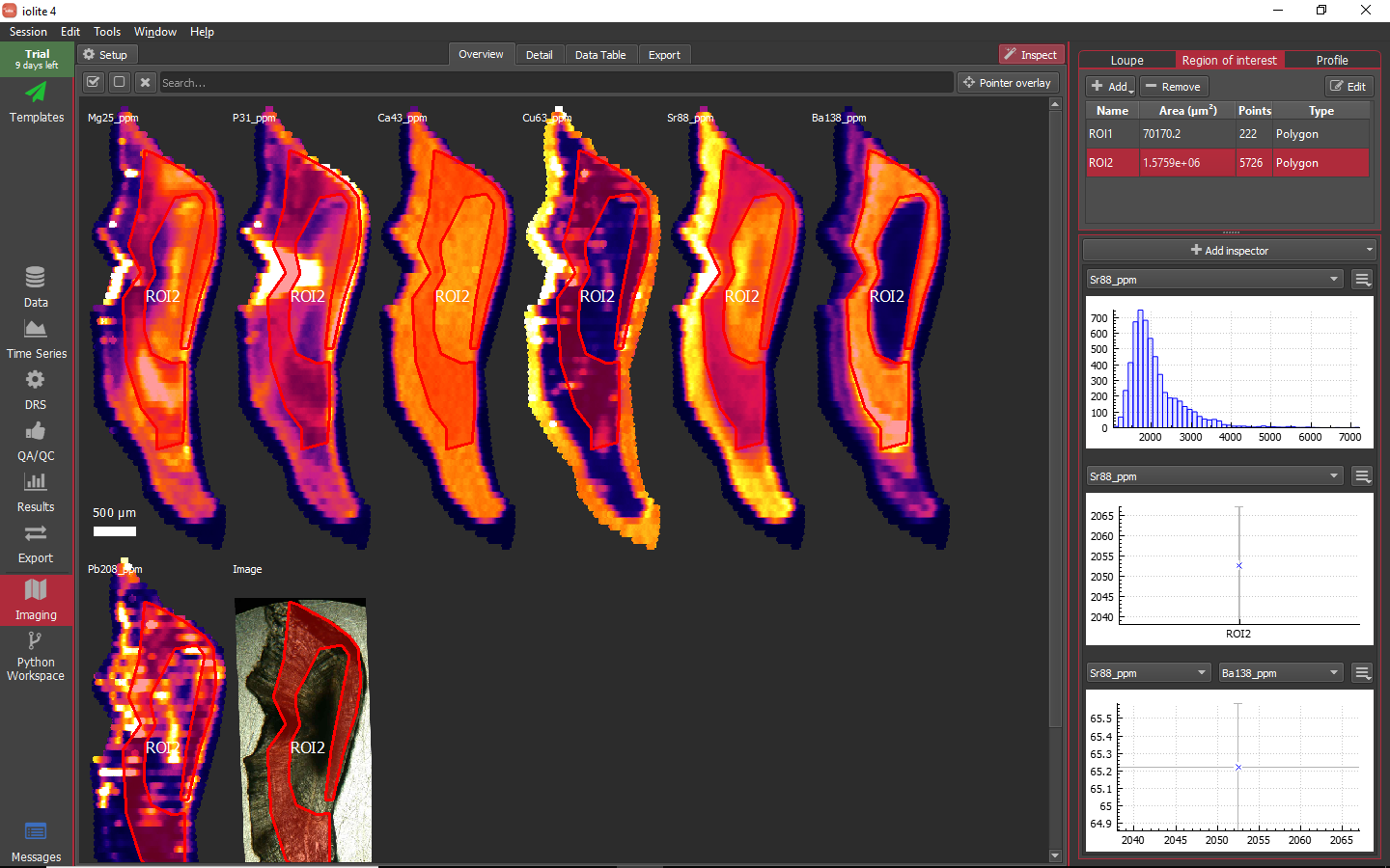
You can select multiple ROIs in the table to see how they plot on whichever inspectors you have configured as shown below.

One alternative to drawing an ROI is to define it using a set of criteria. When you select From criteria from the Add drop-down menu you are presented with a dialog as below.

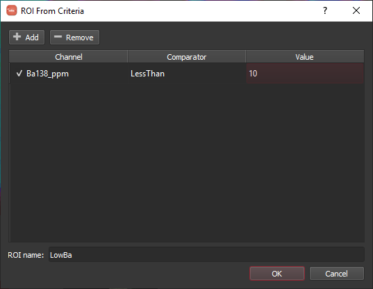
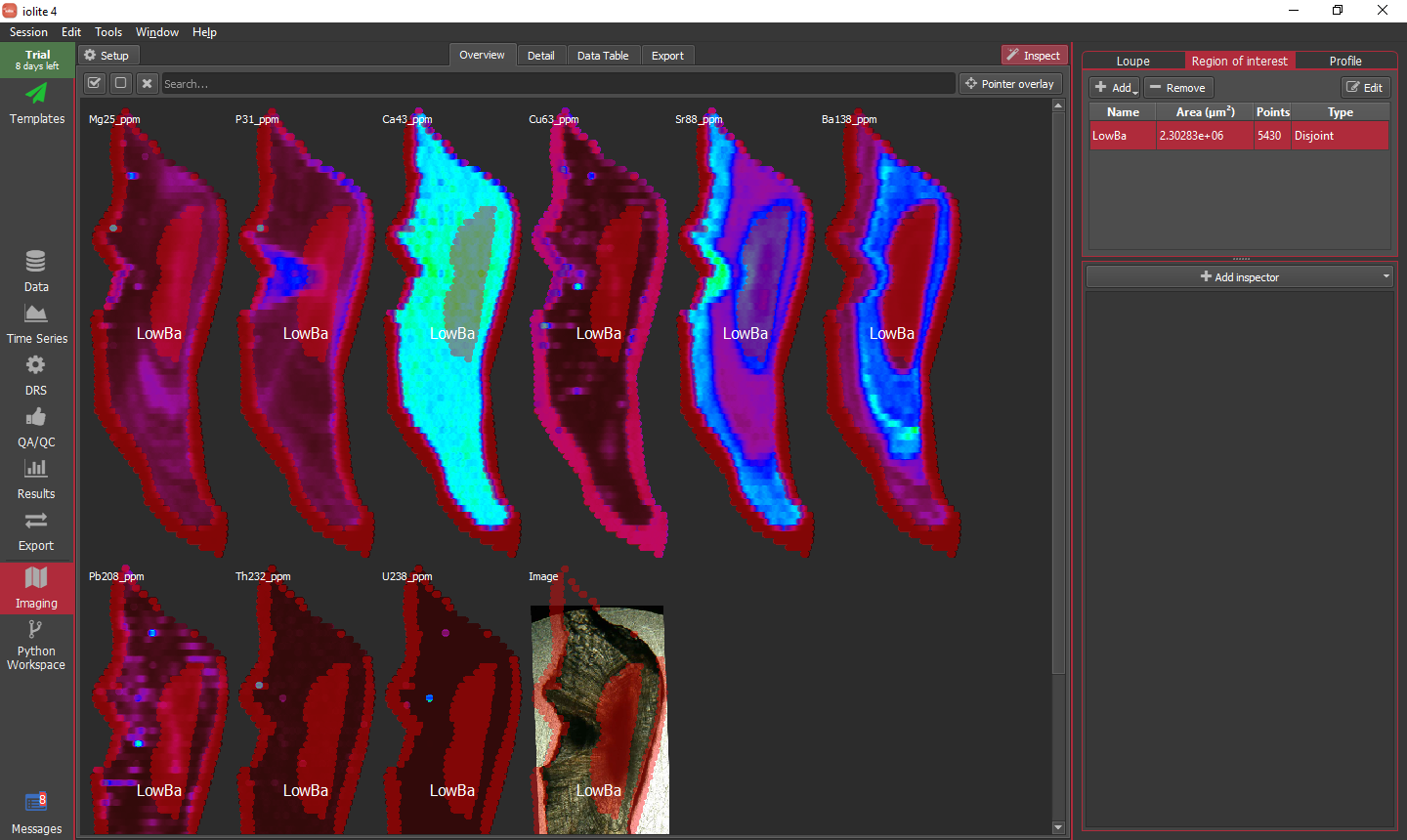
As an example, let's try to make an ROI capturing the Ba low in the middle of the otolith. As a first attempt, we can add a single criterion to the list by clicking the Add button and setting the channel, comparator and value to Ba138_ppm, LessThan and 10, respectively. Enter a name for the ROI and click OK. In doing so, we find that it does pick out the central Ba low, but also picks up much of the otolith rim where all of the signals are dropping off as shown below.

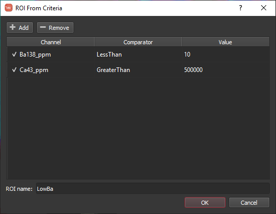
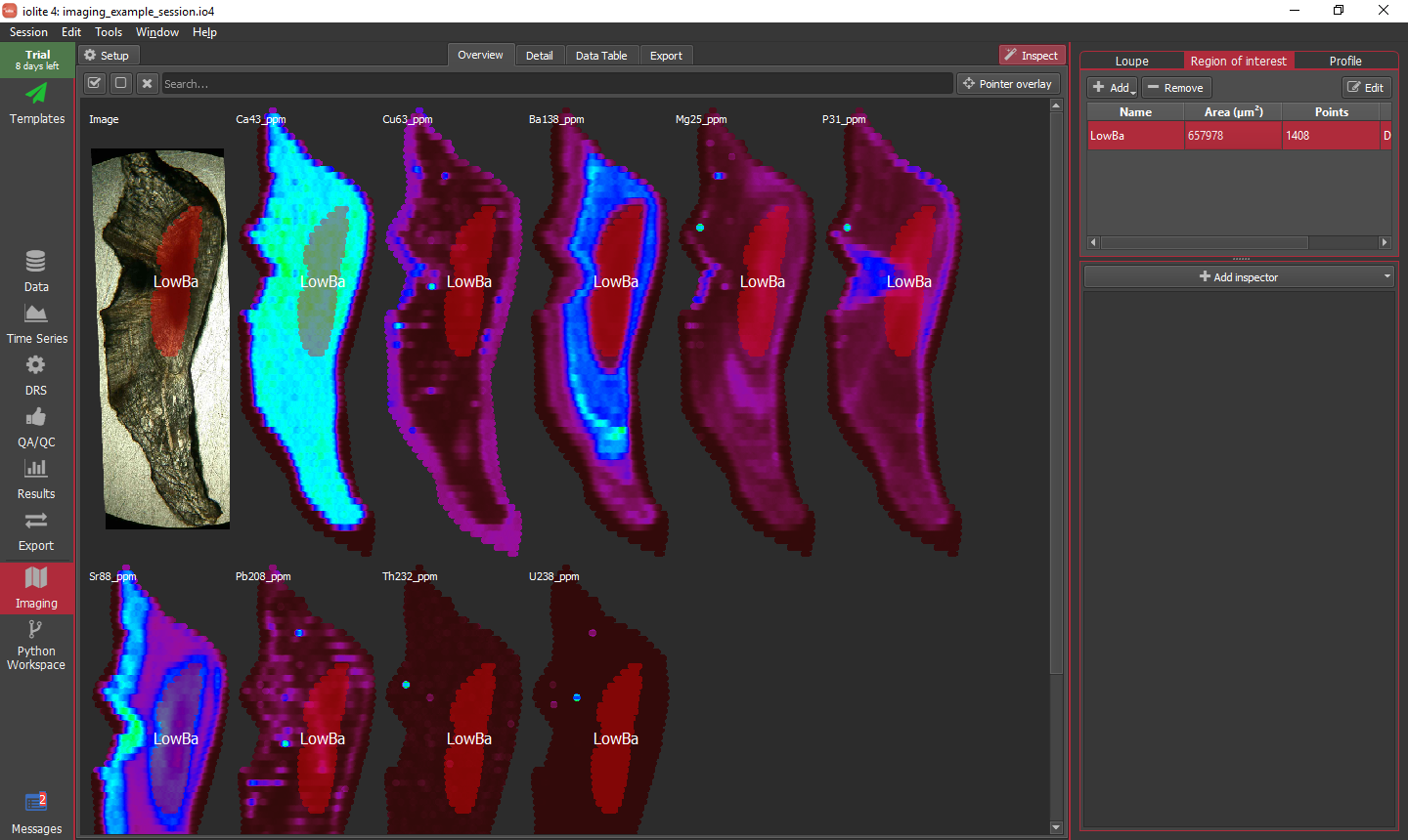
Returning to our ROI criteria by clicking the Edit button, we can add additional criteria to better define our intended area. To get rid of this bit of data around the edge, we can add a second criterion with the channel, comparator and value set to Ca43_ppm, GreaterThan, and 500000, respectively. This combination of criteria yields the intended region as shown below.

In some instances, depending on the nature of the data, it may be difficult or impossible to capture the region of interest using criteria. An alternative tool is to 'grow' an ROI from a seed. To initiate the process select From seed from the ROI Add menu. When you select this menu item a message overlay is shown along the bottom of the window tell you to click on an image to set the seed point. Once you do as asked, a dialog will appear as below.

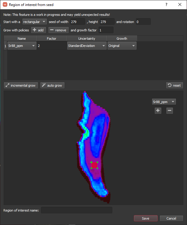
For this example, I clicked in the lower-middle Sr low area and am going to grow to fill that Sr low. It will start with a seed area around the point you clicked defined by a rectangle and geometry based on the spot size. This default should work fine here. Next, we add a growth policy by clicking the add button. A row will appear in the table. Since we want to grow based on Sr, we should select Sr88_ppm in the Name column, and the defaults should be ok for the rest. When things are setup, you can click the auto grow button highlighted below. Once it has grown (this can take some time as it is quite computationally intensive), you can specify a name along the bottom and click Save.

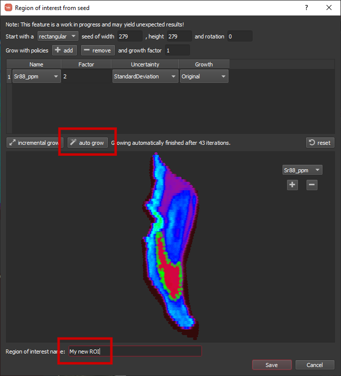
Hint

You can click and drag to move the seed rectangle or ellipse.

Hint

If things did not go expected, you can click the reset button to undo the growth and change some parameters before trying again.

Hint

You can merge and subdivide ROI using a right-click context menu.

Hint

Regions of interest that are created from a seed end up as a polygon-type ROI, which means when you click edit you are able to move and delete vertices.

Creating profiles

Profiles can be created in the Profile tool much like ROIs. When the add button is clicked, an overlay message will appear along the bottom of the window telling you to click to add vertices and double click to add the last vertex. Once the last vertex is added, a dialog will pop up asking you to name the profile. One important concept regarding the way profiles are handled in iolite 4 is that profiles are constructed as a series of sub-ROI or slices along the profile. The dimensions of each sub-ROI can be specified in the Slice area column of the profiles table by double clicking and typing in the dimensions, e.g. '50 x 200'. When a profile is being visualized in an inspector it is the data for these sub-ROI that are displayed.

As an example, I have created a profile across the otolith capturing the highs and lows. By default the slice area will be '100 x 300', but here I have changed that to '75 x 200'. In the inspectors panel, I have a simple stats plot showing the Sr concentration along the profile and an X-Y plot showing Sr vs Ba.

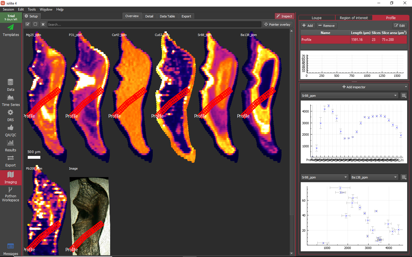
Hint

Profiles can be edited by selecting the profile you want to edit in the table, clicking the Edit button, and click + dragging to move vertices or clicking and then pressing delete to remove a vertex.

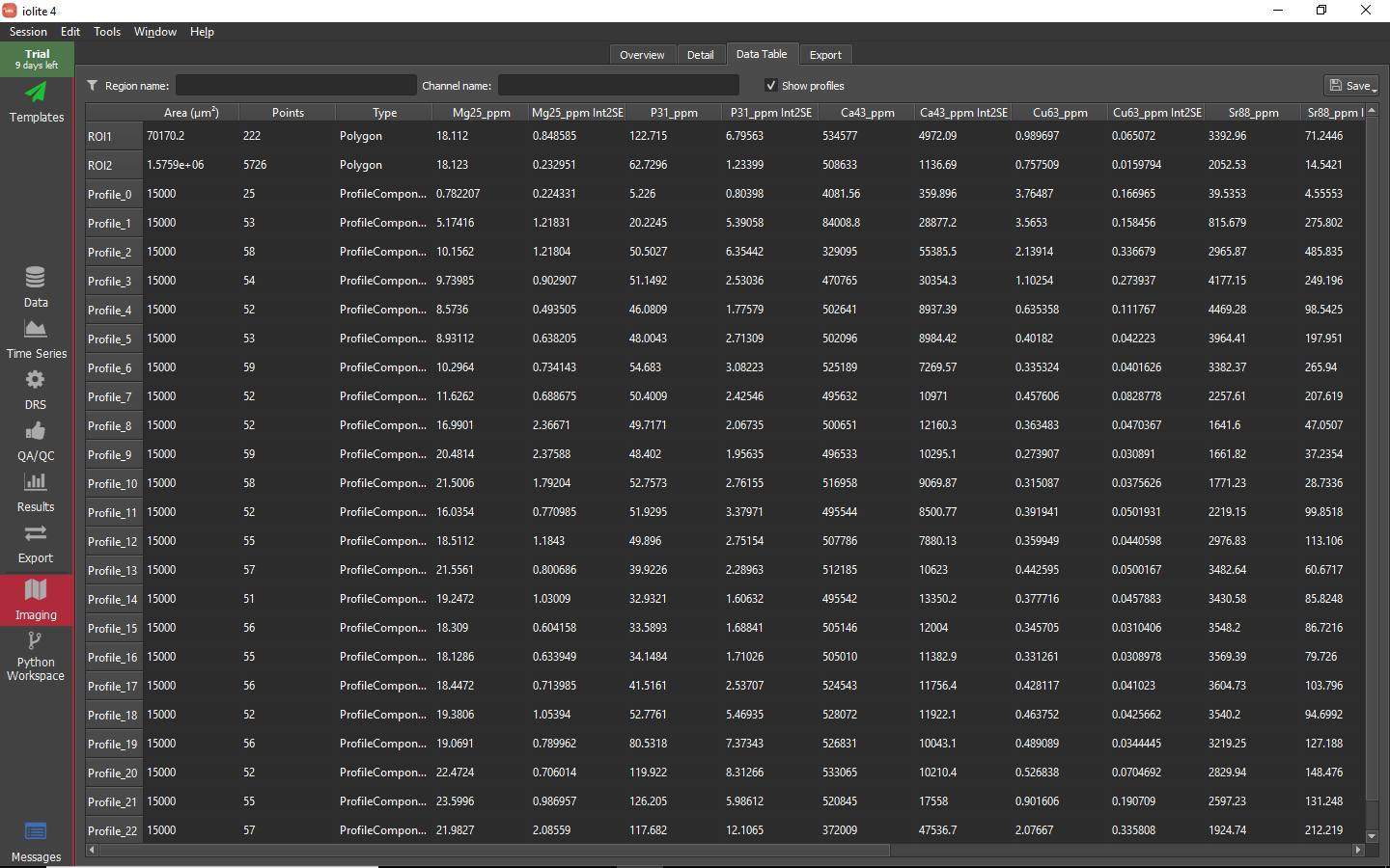
Perusing the data

Before exporting the data

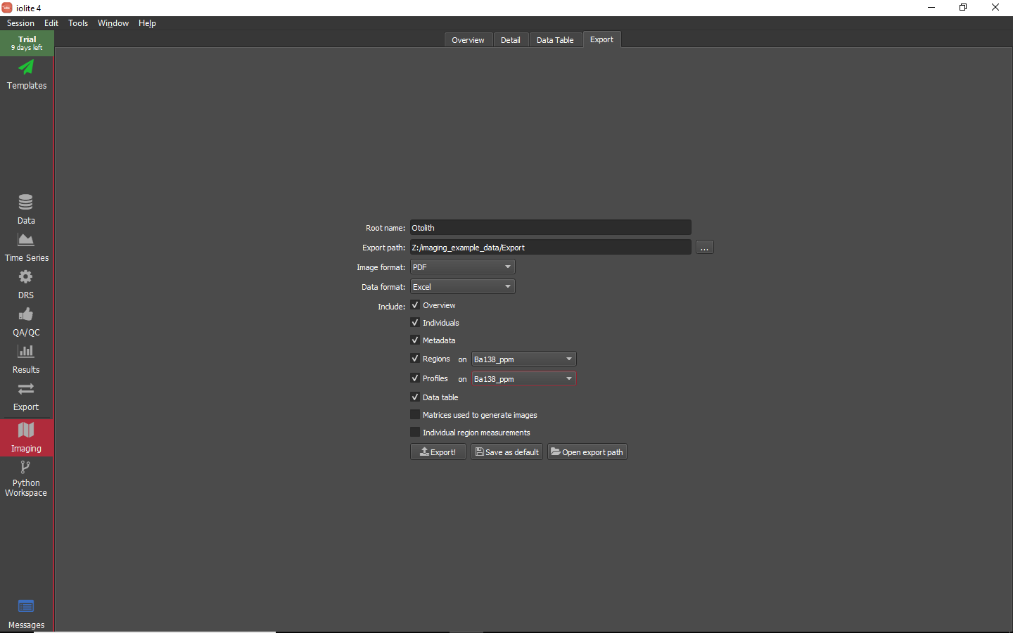
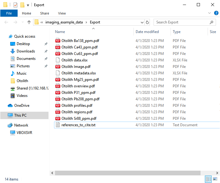
Exporting images and data

There are several options available to export imaging data. What you export will depend on personal preference and the intended use of the image data. As an example, for this experiment